19 Inference for a single mean
Focusing now on Statistical Inference for numerical data, again, we will revisit and expand upon the foundational aspects of hypothesis testing from Chapter 11.
The important data structure for this chapter is a numeric response variable (that is, the outcome is quantitative). The four data structures we detail are one numeric response variable, one numeric response variable which is a difference across a pair of observations, a numeric response variable broken down by a binary explanatory variable, and a numeric response variable broken down by an explanatory variable that has two or more levels. When appropriate, each of the data structures will be analyzed using the three methods from Chapter 11, Chapter 12, and Chapter 13: randomization test, bootstrapping, and mathematical models, respectively.
As we build on the inferential ideas, we will visit new foundational concepts in statistical inference. One key new idea rests in estimating how the sample mean (as opposed to the sample proportion) varies from sample to sample; the resulting value is referred to as the standard error of the mean. We will also introduce a new important mathematical model, the \(t\)-distribution (as the foundation for the \(t\)-test).
In this chapter, we focus on the sample mean (instead of, for example, the sample median or the range of the observations) because of the well-studied mathematical model which describes the behavior of the sample mean. We will not cover mathematical models which describe other statistics, but the bootstrap and randomization techniques described below are immediately extendable to any function of the observed data. The sample mean will be calculated in one group, two paired groups, two independent groups, and many groups settings. The techniques described for each setting will vary slightly, but you will be well served to find the structural similarities across the different settings.
Similar to how we can model the behavior of the sample proportion \(\hat{p}\) using a normal distribution, the sample mean \(\bar{x}\) can also be modeled using a normal distribution when certain conditions are met. However, we’ll soon learn that a new distribution, called the \(t\)-distribution, is more useful when working with the sample mean. We’ll first learn about this new distribution, then we’ll use it for confidence intervals and hypothesis tests for the mean.
19.1 Bootstrap confidence interval for a mean
Consider a situation where you want to know whether you should buy a franchise of the used car store Awesome Autos. As part of your planning, you’d like to know for how much an average car from Awesome Autos sells. In order to go through the example more clearly, let’s say that you are only able to randomly sample five cars from Awesome Auto. (If this were a real example, you would surely be able to take a much larger sample size, possibly even being able to measure the entire population!)
19.1.1 Observed data
Figure 19.1 shows a (small) random sample of observations from Awesome Auto. The actual cars as well as their selling price are shown.
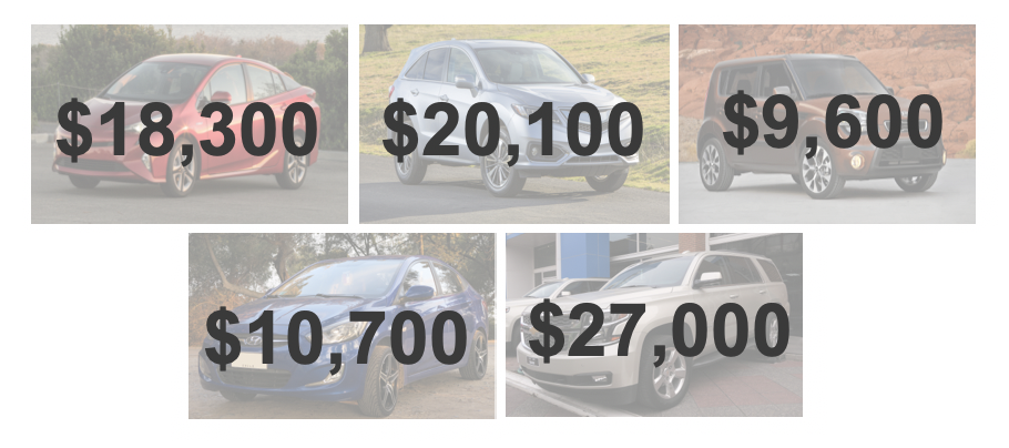
The sample average car price of $17140.00 is a first guess at the price of the average car price at Awesome Auto. However, as a student of statistics, you understand that one sample mean based on a sample of five observations will not necessarily equal the true population average car price for all the cars at Awesome Auto. Indeed, you can see that the observed car prices vary with a standard deviation of $7170.29, and surely the average car price would be different if a different sample of size five had been taken from the population. Fortunately, as it did in previous chapters for the sample proportion, bootstrapping will approximate the variability of the sample mean from sample to sample.
19.1.2 Variability of the statistic
As with the inferential ideas covered in Chapter 11, Chapter 12, and Chapter 13, the inferential analysis methods in this chapter are grounded in quantifying how one dataset differs from another when they are both taken from the same population. To repeat, the idea is that we want to know how datasets differ from one another, but we aren’t ever going to take more than one sample of observations. It does not make sense to take repeated samples from the same population because if you have the ability to take more samples, a larger sample size will benefit you more than taking two samples from the population. Instead, of taking repeated samples from the actual population, we use bootstrapping to measure how the samples behave under an estimate of the population.
As mentioned previously, to get a sense of the cars at Awesome Auto, you take a sample of five cars from the Awesome Auto branch near you as a way to gauge the price of the cars being sold. Figure 19.2 shows how the unknown population of car prices at Awesome Auto can be approximated using the sample.
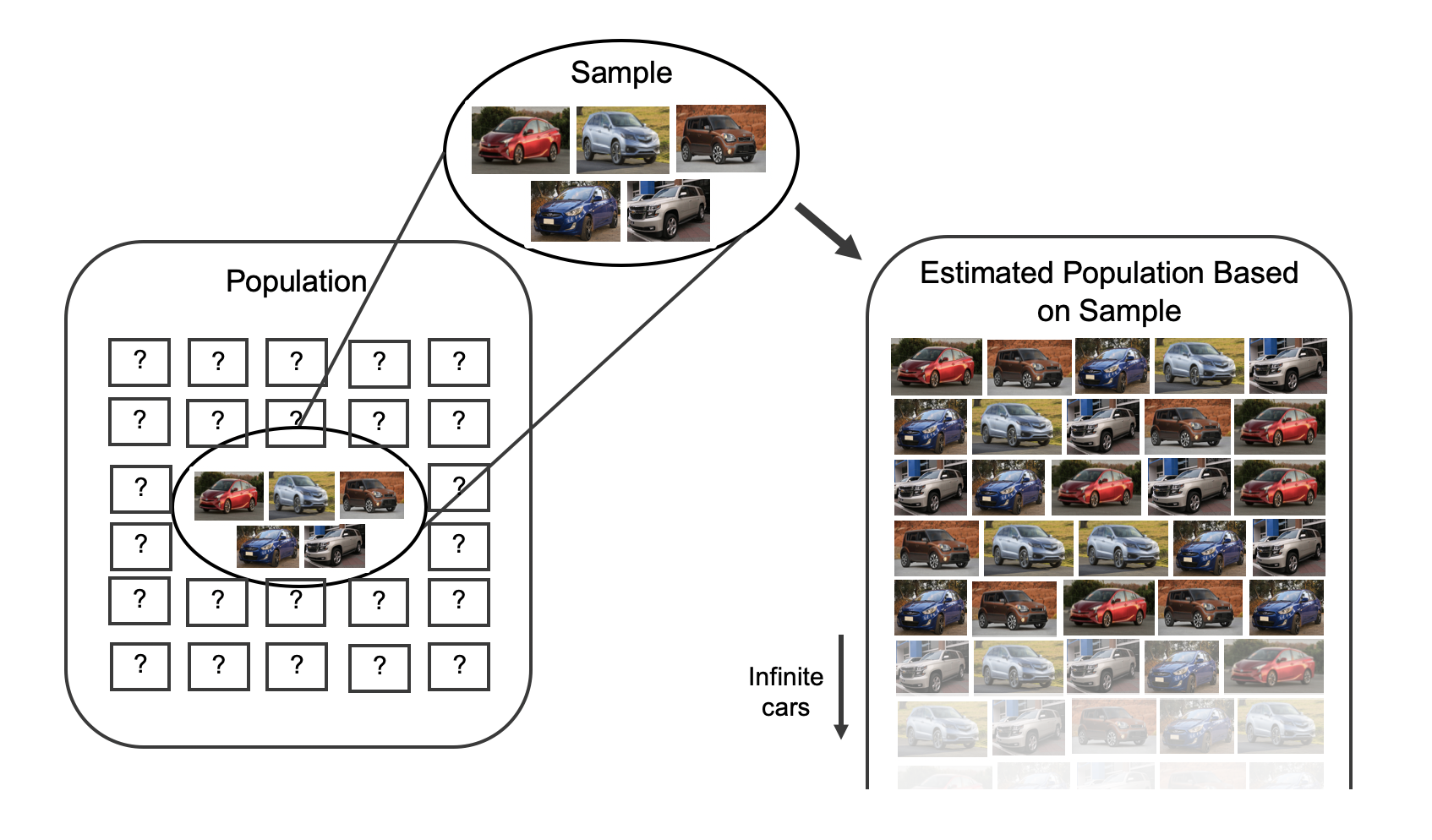
By taking repeated samples from the estimated population, the variability from sample to sample can be observed. In Figure 12.2 the repeated bootstrap samples are seen to be different both from each other and from the original population. Recall that the bootstrap samples were taken from the same (estimated) population, and so the differences in bootstrap samples are due entirely to natural variability in the sampling procedure. For the situation at hand where the sample mean is the statistic of interest, the variability from sample to sample can be seen in Figure 19.3.
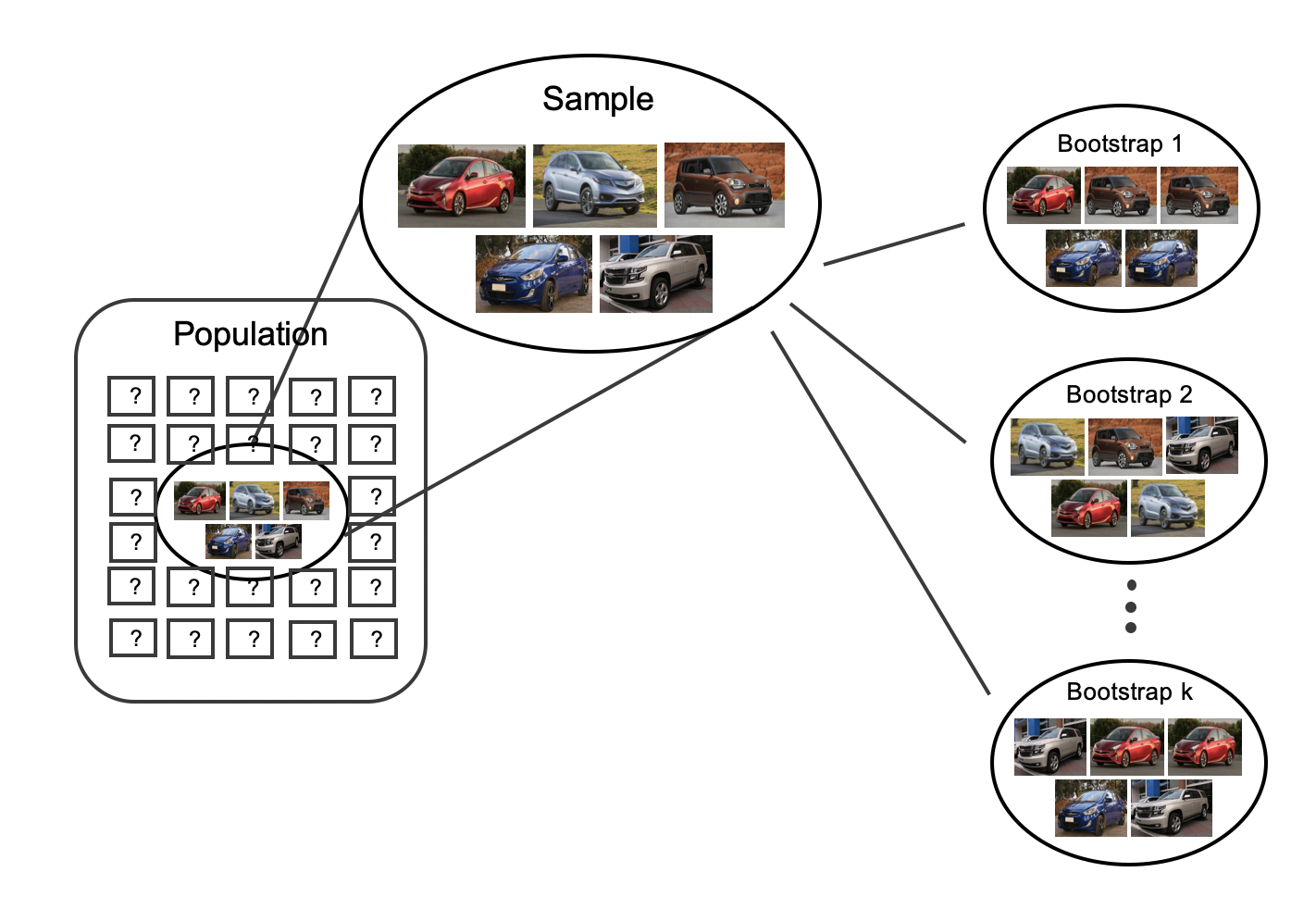
By summarizing each of the bootstrap samples (here, using the sample mean), we see, directly, the variability of the sample mean, \(\bar{x},\) from sample to sample. The distribution of \(\bar{x}_{bs}\) for the Awesome Auto cars is shown in Figure 19.4.
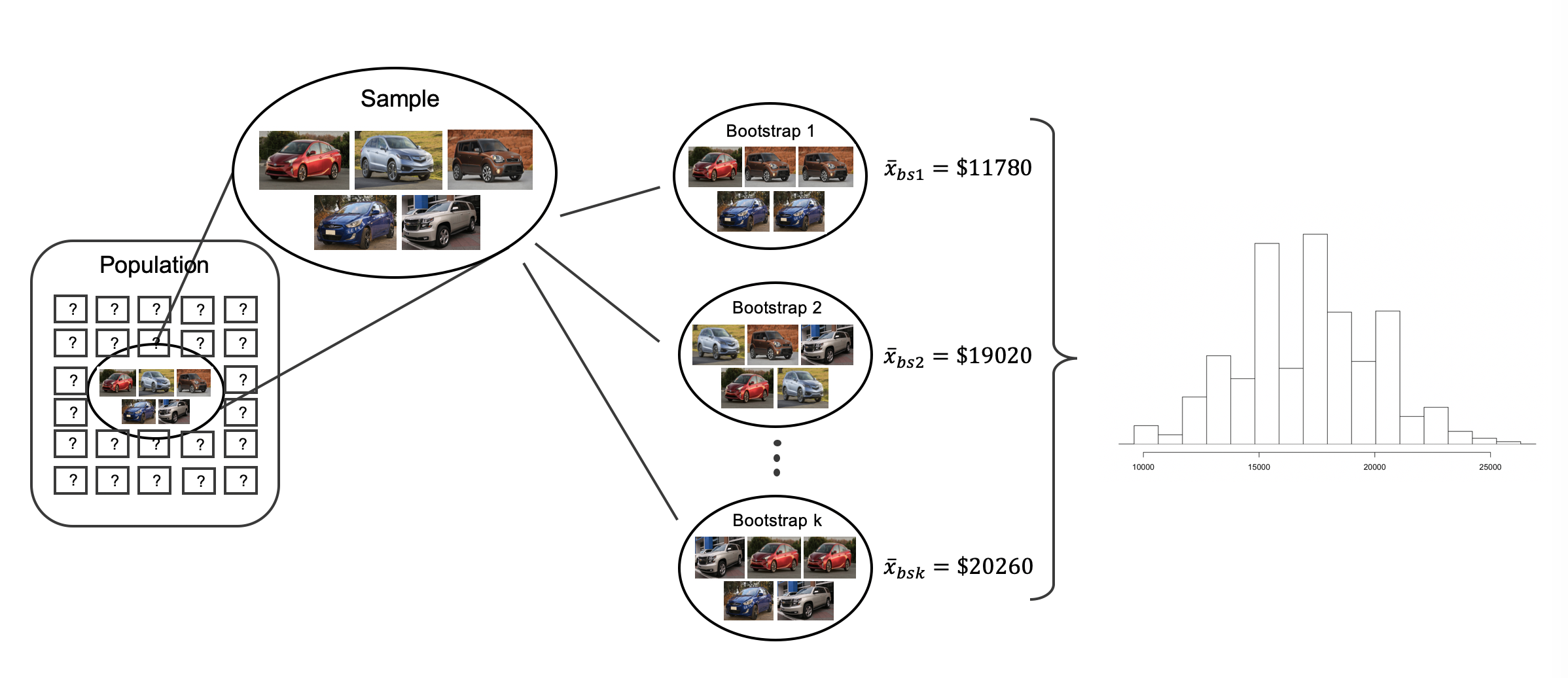
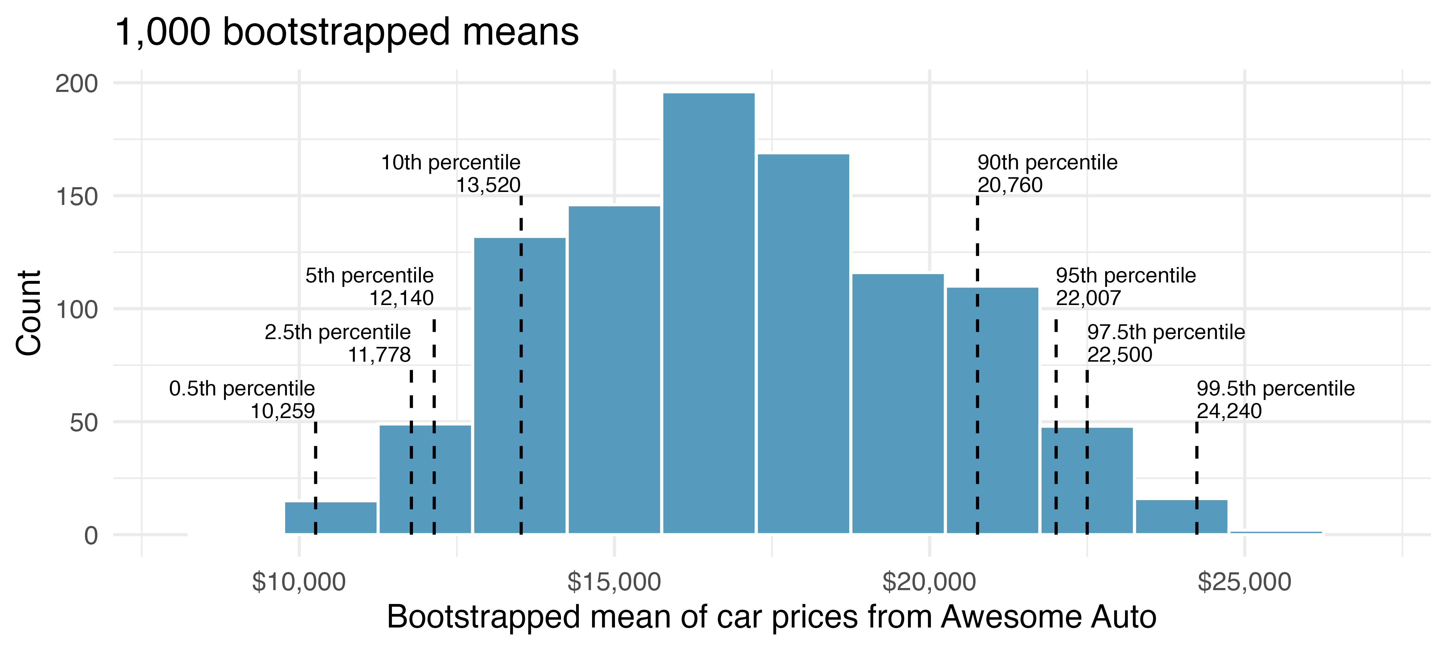
Figure 19.5 summarizes one thousand bootstrap samples in a histogram of the bootstrap sample means. The bootstrapped average car prices vary from about $10,000 to $25,000. The bootstrap percentile confidence interval is found by locating the middle 90% (for a 90% confidence interval) or a 95% (for a 95% confidence interval) of the bootstrapped statistics.
Using Figure 19.5, find the 90% and 95% bootstrap percentile confidence intervals for the true average price of a car from Awesome Auto.
A 90% confidence interval is $12,140 to $22,007. The conclusion is that we are 90% confident that the true average car price at Awesome Auto lies somewhere between $12,140 and $22,007.
A 95% confidence interval is $11,778 to $22,500. The conclusion is that we are 95% confident that the true average car price at Awesome Auto lies somewhere between $11,778 to $22,500.
19.1.3 Bootstrap SE confidence interval
As seen in Section 17.2, another method for creating bootstrap confidence intervals directly uses a calculation of the variability of the bootstrap statistics (here, the bootstrap means). If the bootstrap distribution is relatively symmetric and bell-shaped, then the 95% bootstrap SE confidence interval can be constructed with the formula familiar from the mathematical models in previous chapters:
\[\mbox{point estimate} \pm 2 \cdot SE_{BS}\] The number 2 is an approximation connected to the “95%” part of the confidence interval (remember the 68-95-99.7 rule). As will be seen in Section 19.2, a new distribution (the \(t\)-distribution) will be applied to most mathematical inference on numerical variables. However, because bootstrapping is not grounded in the same theory as the mathematical approach given in this text, we stick with the standard normal quantiles (in R use the function qnorm() to find normal percentiles other than 95%) for different confidence percentages.1
Explain how the standard error (SE) of the bootstrapped means is calculated and what it is measuring.
The SE of the bootstrapped means measures how variable the means are from resample to resample. The bootstrap SE is a good approximation to the SE of means as if we had taken repeated samples from the original population (which we agreed isn’t something we would do because of wasted resources).
Logistically, we can find the standard deviation of the bootstrapped means using the same calculations from Chapter 5. That is, the bootstrapped means are the individual observations about which we measure the variability.
Although we won’t spend a lot of energy on this concept, you may be wondering some of the differences between a standard error and a standard deviation. The standard error describes how a statistic (e.g., sample mean or sample proportion) varies from sample to sample. The standard deviation can be thought of as a function applied to any list of numbers which measures how far those numbers vary from their own average. So, you can have a standard deviation calculated on a column of dog heights or a standard deviation calculated on a column of bootstrapped means from the resampled data. Note that the standard deviation calculated on the bootstrapped means is referred to as the bootstrap standard error of the mean.
It turns out that the standard deviation of the bootstrapped means from Figure 19.5 is $2,891.87 (a value which is an excellent approximation for the standard error of sample means if we were to take repeated samples from the population). (Note: in R the calculation was done using the function sd().) The average of the observed prices is $17,140, and we will consider the sample average to be the best guess point estimate for \(\mu.\) Find and interpret the confidence interval for \(\mu\) (the true average cost of a car at Awesome Auto) using the bootstrap SE confidence interval formula.2
Compare and contrast the two different 95% confidence intervals for \(\mu\) created by finding the percentiles of the bootstrapped means and created by finding the SE of the bootstrapped means. Do you think the intervals should be identical?
- Percentile interval: ($11,778, $22,500)
- SE interval: ($11,356.26, $22,923.74)
The intervals were created using different methods, so it is not surprising that they are not identical. However, we are pleased to see that the two methods provide very similar interval approximations. The technical details surrounding which data structures are best for percentile intervals and which are best for SE intervals is beyond the scope of this text. However, the larger the samples are, the better (and closer) the interval estimates will be.
19.1.4 Bootstrap percentile confidence interval for a standard deviation
Suppose that we want to understand how variable the prices of the cars are at Awesome Auto. That is, your interest is no longer in the average car price but in the standard deviation of the prices of all cars at Awesome Auto, \(\sigma.\) You may have already realized that the sample standard deviation, \(s,\) will work as a good point estimate for the parameter of interest: the population standard deviation, \(\sigma.\) The point estimate of the five observations is calculated to be \(s = \$7,170.286.\) While \(s = \$7,170.286\) might be a good guess for \(\sigma,\) we prefer to have an interval estimate for the parameter of interest. Although there is a mathematical model which describes how \(s\) varies from sample to sample, the mathematical model will not be presented in this text. Instead, bootstrapping can be used to find a confidence interval for the parameter \(\sigma.\) Using the same technique as presented for a confidence interval for \(\mu,\) here we find the bootstrap percentile confidence interval for \(\sigma.\)
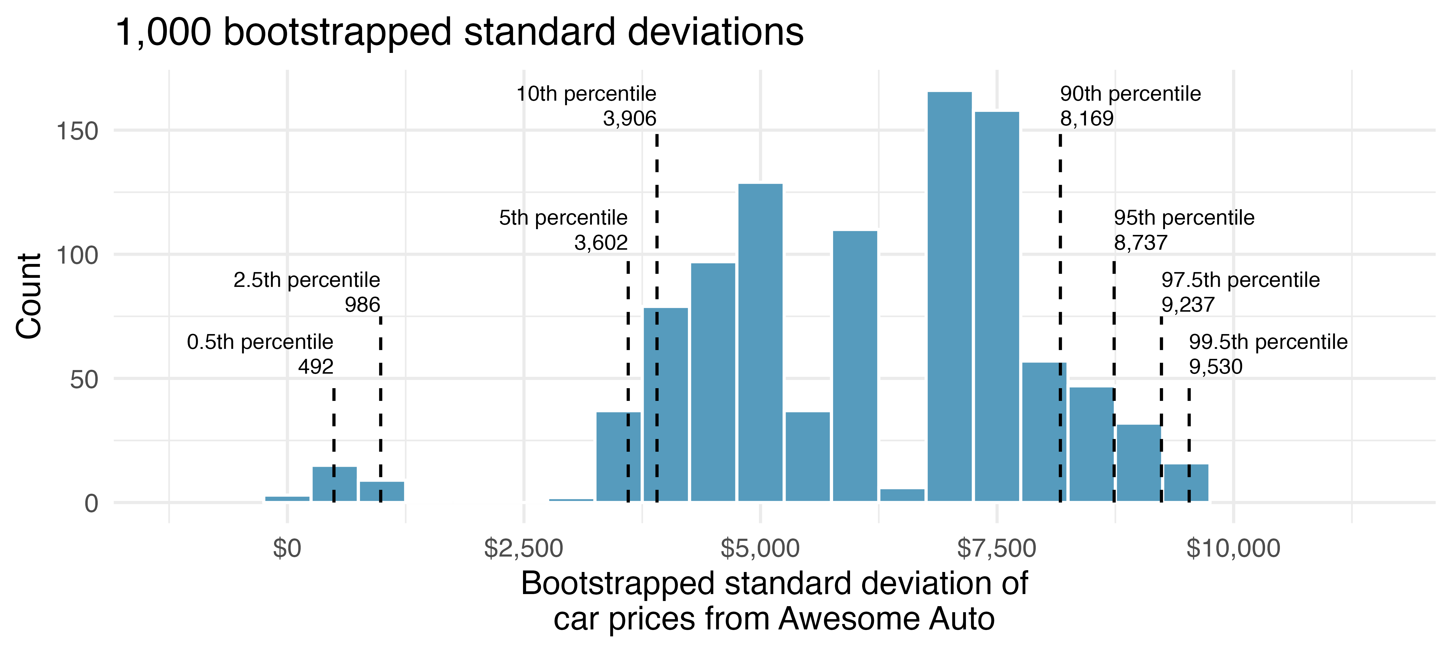
Describe the bootstrap distribution for the standard deviation shown in Figure 19.6.
The distribution is skewed left and centered near $7,170.286, which is the point estimate from the original data. Most observations in this distribution lie between $0 and $10,000.
Using Figure 19.6, find and interpret a 90% bootstrap percentile confidence interval for the population standard deviation for car prices at Awesome Auto.3
19.1.5 Bootstrapping is not a solution to small sample sizes!
The example presented above is done for a sample with only five observations. As with analysis techniques that build on mathematical models, bootstrapping works best when a large random sample has been taken from the population. Bootstrapping is a method for capturing the variability of a statistic when the mathematical model is unknown (it is not a method for navigating small samples). As you might guess, the larger the random sample, the more accurately that sample will represent the population of interest.
19.2 Mathematical model for a mean
As with the sample proportion, the variability of the sample mean is well described by the mathematical theory given by the Central Limit Theorem. However, because of missing information about the inherent variability in the population (\(\sigma\)), a \(t\)-distribution is used in place of the standard normal when performing hypothesis test or confidence interval analyses.
19.2.1 Mathematical distribution of the sample mean
The sample mean tends to follow a normal distribution centered at the population mean, \(\mu,\) when certain conditions are met. Additionally, we can compute a standard error for the sample mean using the population standard deviation \(\sigma\) and the sample size \(n.\)
Central Limit Theorem for the sample mean.
When we collect a sufficiently large sample of \(n\) independent observations from a population with mean \(\mu\) and standard deviation \(\sigma,\) the sampling distribution of \(\bar{x}\) will be nearly normal with
\[\text{Mean} = \mu \qquad \text{Standard Error }(SE) = \frac{\sigma}{\sqrt{n}}\]
Before diving into confidence intervals and hypothesis tests using \(\bar{x},\) we first need to cover two topics:
- When we modeled \(\hat{p}\) using the normal distribution, certain conditions had to be satisfied. The conditions for working with \(\bar{x}\) are a little more complex, and below, we will discuss how to check conditions for inference using a mathematical model.
- The standard error is dependent on the population standard deviation, \(\sigma.\) However, we rarely know \(\sigma,\) and instead we must estimate it. Because this estimation is itself imperfect, we use a new distribution called the \(t\)-distribution to fix this problem.
19.2.2 Evaluating the two conditions required for modeling \(\bar{x}\)
Two conditions are required to apply the Central Limit Theorem for a sample mean \(\bar{x}:\)
Independence. The sample observations must be independent. The most common way to satisfy this condition is when the sample is a simple random sample from the population. If the data come from a random process, analogous to rolling a die, this would also satisfy the independence condition.
Normality. When a sample is small, we also require that the sample observations come from a normally distributed population. We can relax this condition more and more for larger and larger sample sizes. This condition is vague, making it difficult to evaluate, so next we introduce a couple rules of thumb to checking it.
General rule for performing the normality check.
There is no perfect way to check the normality condition, so instead we use two general rules based on the number and magnitude of extreme observations. Note, it often takes practice to get a sense for whether a normal approximation is appropriate.
- Small \(n\): If the sample size \(n\) is small and there are no clear outliers in the data, then we typically assume the data come from a nearly normal distribution to satisfy the condition.
- Large \(n\): If the sample size \(n\) is large and there are no particularly extreme outliers, then we typically assume the sampling distribution of \(\bar{x}\) is nearly normal, even if the underlying distribution of individual observations is not.
Some guidelines for determining whether \(n\) is considered small or large are as follows: slight skew is okay for sample sizes of 15, moderate skew for sample sizes of 30, and strong skew for sample sizes of 60.
In this first course in statistics, you aren’t expected to develop perfect judgment on the normality condition. However, you are expected to be able to handle clear cut cases based on the rules of thumb.4
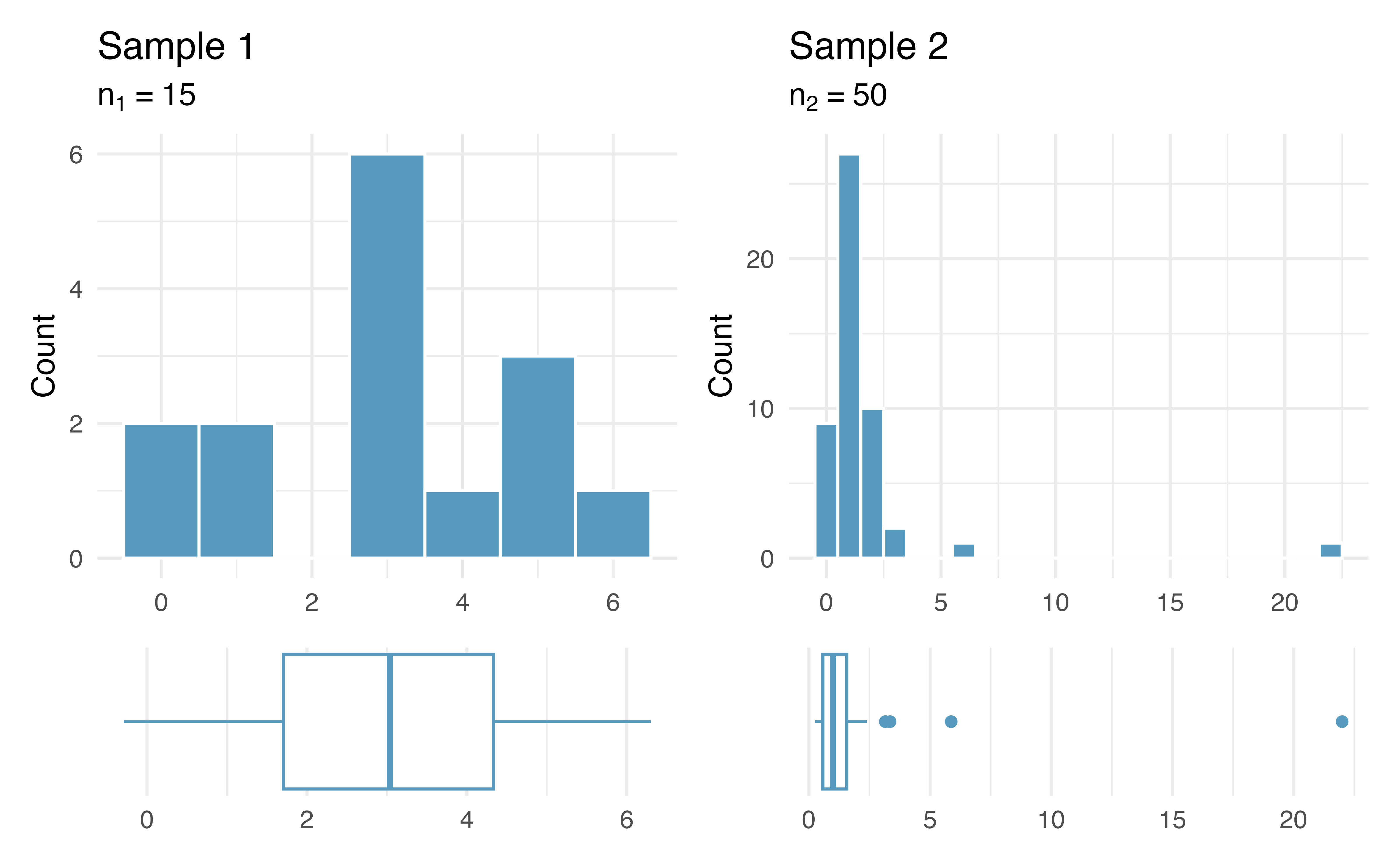
Consider the four plots provided in Figure 19.7 that come from simple random samples from different populations. Their sample sizes are \(n_1 = 15\) and \(n_2 = 50.\)
Are the independence and normality conditions met in each case?
Each samples is from a simple random sample of its respective population, so the independence condition is satisfied. Let’s next check the normality condition for each using the rule of thumb.
The first sample has fewer than 30 observations, so we are watching for any clear outliers. None are present; while there is a small gap in the histogram on the right, this gap is small and over 20% of the observations in this small sample are represented to the left of the gap, so we can hardly call these clear outliers. With no clear outliers, the normality condition can be reasonably assumed to be met.
The second sample has a sample size greater than 30 and includes an outlier that appears to be roughly 5 times further from the center of the distribution than the next furthest observation. This is an example of a particularly extreme outlier, so the normality condition would not be satisfied.
It’s often helpful to also visualize the data using a box plot to assess skewness and existence of outliers. The box plots provided underneath each histogram confirms our conclusions that the first sample does not have any outliers and the second sample does, with one outlier being particularly more extreme than the others.
In practice, it’s typical to also do a mental check to evaluate whether we have reason to believe the underlying population would have moderate skew (if \(n < 30)\) or have particularly extreme outliers \((n \geq 30)\) beyond what we observe in the data. For example, consider the number of followers for each individual account on Twitter, and then imagine this distribution. The large majority of accounts have built up a couple thousand followers or fewer, while a relatively tiny fraction have amassed tens of millions of followers, meaning the distribution is extremely skewed. When we know the data come from such an extremely skewed distribution, it takes some effort to understand what sample size is large enough for the normality condition to be satisfied.
19.2.3 Introducing the t-distribution
In practice, we cannot directly calculate the standard error for \(\bar{x}\) since we do not know the population standard deviation, \(\sigma.\) We encountered a similar issue when computing the standard error for a sample proportion, which relied on the population proportion, \(p.\) Our solution in the proportion context was to use the sample value in place of the population value when computing the standard error. We’ll employ a similar strategy for computing the standard error of \(\bar{x},\) using the sample standard deviation \(s\) in place of \(\sigma:\)
\[SE = \frac{\sigma}{\sqrt{n}} \approx \frac{s}{\sqrt{n}}\]
This strategy tends to work well when we have a lot of data and can estimate \(\sigma\) using \(s\) accurately. However, the estimate is less precise with smaller samples, and this leads to problems when using the normal distribution to model \(\bar{x}.\)
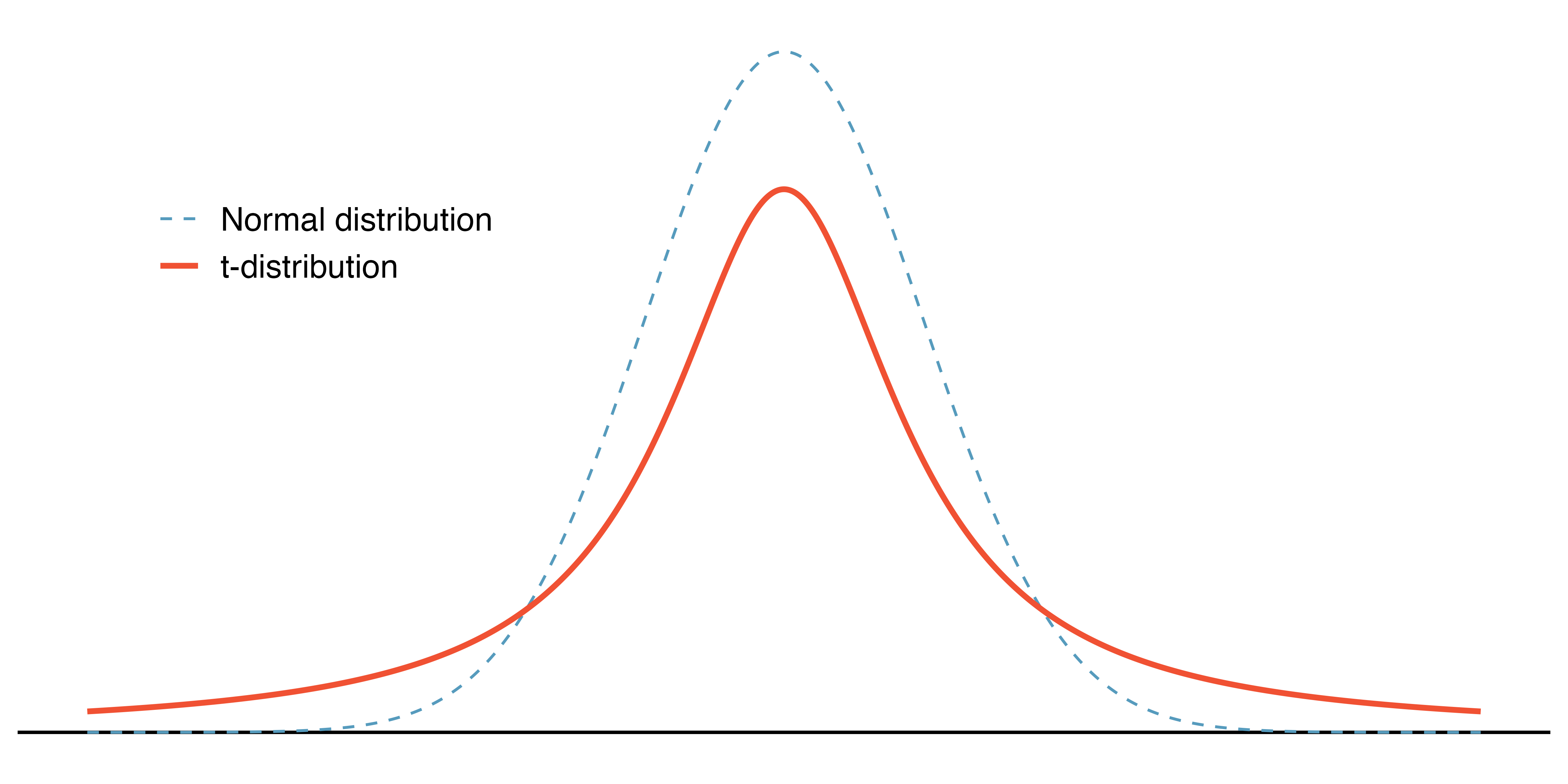
We’ll find it useful to use a new distribution for inference calculations called the \(t\)-distribution. A \(t\)-distribution, shown as a solid line in Figure 19.8, has a bell shape. However, its tails are thicker than the normal distribution’s, meaning observations are more likely to fall beyond two standard deviations from the mean than under the normal distribution.
The extra thick tails of the \(t\)-distribution are exactly the correction needed to resolve the problem (due to extra variability of the T score) of using \(s\) in place of \(\sigma\) in the \(SE\) calculation.
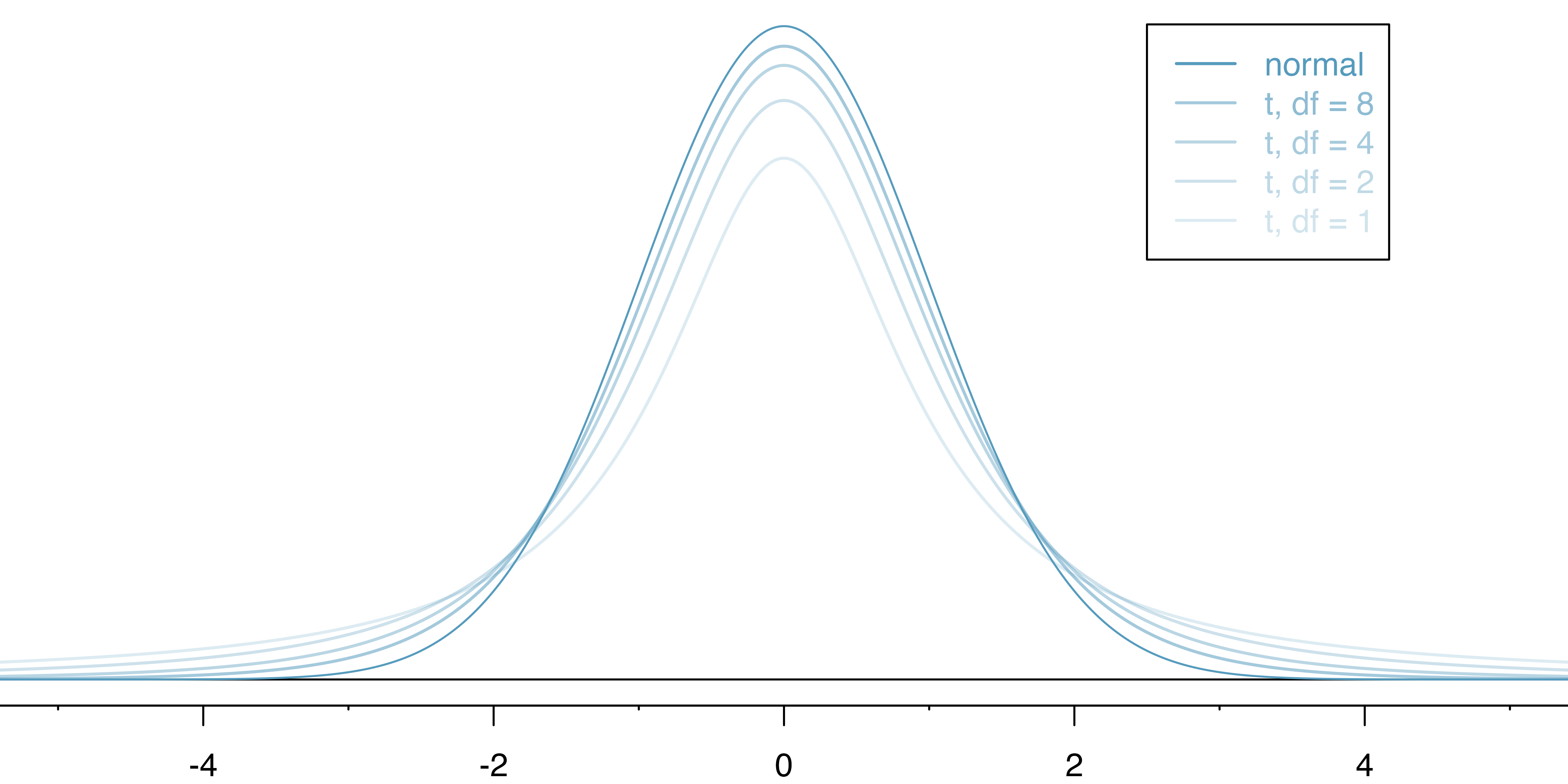
The \(t\)-distribution is always centered at zero and has a single parameter: degrees of freedom. The degrees of freedom describes the precise form of the bell-shaped \(t\)-distribution. Several \(t\)-distributions are shown in Figure 19.9 in comparison to the normal distribution. Similar to the Chi-square distribution, the shape of the \(t\)-distribution also depends on the degrees of freedom.
In general, we’ll use a \(t\)-distribution with \(df = n - 1\) to model the sample mean when the sample size is \(n.\) That is, when we have more observations, the degrees of freedom will be larger and the \(t\)-distribution will look more like the standard normal distribution; when the degrees of freedom is about 30 or more, the \(t\)-distribution is nearly indistinguishable from the normal distribution.
Degrees of freedom: df.
The degrees of freedom describes the shape of the \(t\)-distribution. The larger the degrees of freedom, the more closely the distribution approximates the normal distribution.
When modeling \(\bar{x}\) using the \(t\)-distribution, use \(df = n - 1.\)
The \(t\)-distribution allows us greater flexibility than the normal distribution when analyzing numerical data. In practice, it’s common to use statistical software, such as R, Python, or SAS for these analyses. In R, the function used for calculating probabilities under a \(t\)-distribution is pt() (which should seem similar to previous R functions, pnorm() and pchisq()). Don’t forget that with the \(t\)-distribution, the degrees of freedom must always be specified!
For the examples and guided practices below, you may have to use a table or statistical software to find the answers. We recommend trying the problems so as to get a sense for how the \(t\)-distribution can vary in width depending on the degrees of freedom. No matter the approach you choose, apply your method using the examples below to confirm your working understanding of the \(t\)-distribution.
What proportion of the \(t\)-distribution with 18 degrees of freedom falls below -2.10?
Let’s first draw the picture and shade the area below -2.10.
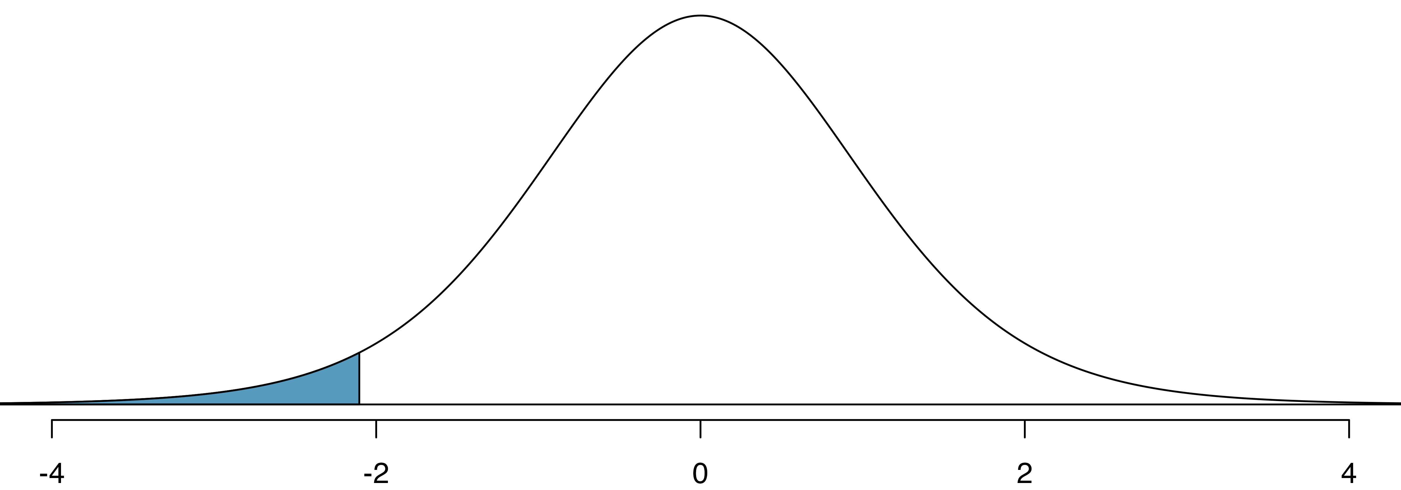
Using statistical software, we can obtain a precise value: 0.0250.
# use pt() to find probability under the t-distribution
pt(-2.10, df = 18)
[1] 0.025What proportion of the 𝑡-distribution with 20 degrees of freedom falls above 1.65?
Note that with 20 degrees of freedom, the \(t\)-distribution is relatively close to the normal distribution. With a normal distribution, this would correspond to about 0.05, so we should expect the \(t\)-distribution to give us a similar value. Using statistical software, we can obtain a precise value: 0.0573.
# use pt() to find probability under the t-distribution
1 - pt(1.65, df = 20)
[1] 0.0573A \(t\)-distribution with 2 degrees of freedom is shown below. Estimate the proportion of the distribution falling more than 3 units from the mean (above or below).
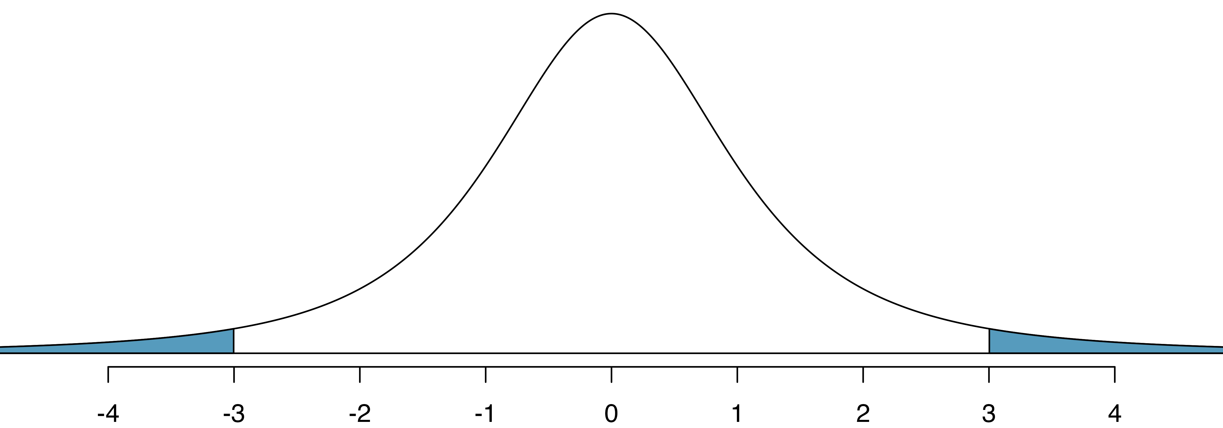
With so few degrees of freedom, the \(t\)-distribution will give a more notably different value than the normal distribution. Under a normal distribution, the area would be about 0.003 using the 68-95-99.7 rule. For a \(t\)-distribution with \(df = 2,\) the area in both tails beyond 3 units totals 0.0955. This area is dramatically different than what we obtain from the normal distribution.
What proportion of the \(t\)-distribution with 19 degrees of freedom falls above -1.79 units? Use your preferred method for finding tail areas.5
19.2.4 One sample t-intervals
Let’s get our first taste of applying the \(t\)-distribution in the context of an example about the mercury content of dolphin muscle. Elevated mercury concentrations are an important problem for both dolphins and other animals, like humans, who occasionally eat them.
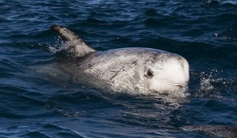
We will identify a confidence interval for the average mercury content in dolphin muscle using a sample of 19 Risso’s dolphins from the Taiji area in Japan. The data are summarized in Table 19.1. The minimum and maximum observed values can be used to evaluate whether there are clear outliers.
| n | Mean | SD | Min | Max |
|---|---|---|---|---|
| 19 | 4.4 | 2.3 | 1.7 | 9.2 |
Are the independence and normality conditions satisfied for this dataset?
The observations are a simple random sample, therefore it is reasonable to assume that the dolphins are independent. The summary statistics in Table 19.1 do not suggest any clear outliers, with all observations within 2.5 standard deviations of the mean. Based on this evidence, the normality condition seems reasonable.
In the normal model, we used \(z^{\star}\) and the standard error to determine the width of a confidence interval. We revise the confidence interval formula slightly when using the \(t\)-distribution:
\[ \begin{aligned} \text{point estimate} \ &\pm\ t^{\star}_{df} \times SE \\ \bar{x} \ &\pm\ t^{\star}_{df} \times \frac{s}{\sqrt{n}} \end{aligned} \]
Using the summary statistics in Table 19.1, compute the standard error for the average mercury content in the \(n = 19\) dolphins.
We plug in \(s\) and \(n\) into the formula: \(SE = \frac{s}{\sqrt{n}} = \frac{2.3}{\sqrt{19}} = 0.528.\)
The value \(t^{\star}_{df}\) is a cutoff we obtain based on the confidence level and the \(t\)-distribution with \(df\) degrees of freedom. That cutoff is found in the same way as with a normal distribution: we find \(t^{\star}_{df}\) such that the fraction of the \(t\)-distribution with \(df\) degrees of freedom within a distance \(t^{\star}_{df}\) of 0 matches the confidence level of interest.
When \(n = 19,\) what is the appropriate degrees of freedom? Find \(t^{\star}_{df}\) for this degrees of freedom and the confidence level of 95%
The degrees of freedom is easy to calculate: \(df = n - 1 = 18.\)
Using statistical software, we find the cutoff where the upper tail is equal to 2.5%: \(t^{\star}_{18} = 2.10.\) The area below -2.10 will also be equal to 2.5%. That is, 95% of the \(t\)-distribution with \(df = 18\) lies within 2.10 units of 0.
Degrees of freedom for a single sample.
If the sample has \(n\) observations and we are examining a single mean, then we use the \(t\)-distribution with \(df=n-1\) degrees of freedom.
Compute and interpret the 95% confidence interval for the average mercury content in Risso’s dolphins.
We can construct the confidence interval as
\[ \begin{aligned} \bar{x} \ &\pm\ t^{\star}_{18} \times SE \\ 4.4 \ &\pm\ 2.10 \times 0.528 \\ (3.29 \ &, \ 5.51) \end{aligned} \] We are 95% confident the average mercury content of muscles in Risso’s dolphins is between 3.29 and 5.51 \(\mu\)g/wet gram, which is considered extremely high.
Calculating a \(t\)-confidence interval for the mean, \(\mu.\)
Based on a sample of \(n\) independent and nearly normal observations, a confidence interval for the population mean is
\[ \begin{aligned} \text{point estimate} \ &\pm\ t^{\star}_{df} \times SE \\ \bar{x} \ &\pm\ t^{\star}_{df} \times \frac{s}{\sqrt{n}} \end{aligned} \]
where \(\bar{x}\) is the sample mean, \(t^{\star}_{df}\) corresponds to the confidence level and degrees of freedom \(df,\) and \(SE\) is the standard error as estimated by the sample.
The FDA’s webpage provides some data on mercury content of fish. Based on a sample of 15 croaker white fish (Pacific), a sample mean and standard deviation were computed as 0.287 and 0.069 ppm (parts per million), respectively. The 15 observations ranged from 0.18 to 0.41 ppm. We will assume these observations are independent. Based on the summary statistics of the data, do you have any objections to the normality condition of the individual observations?6
Estimate the standard error of \(\bar{x} = 0.287\) ppm using the data summaries in the previous Guided Practice. If we are to use the \(t\)-distribution to create a 90% confidence interval for the actual mean of the mercury content, identify the degrees of freedom and \(t^{\star}_{df}.\)
The standard error: \(SE = \frac{0.069}{\sqrt{15}} = 0.0178.\) Degrees of freedom: \(df = n - 1 = 14.\) Since the goal is a 90% confidence interval, we choose \(t_{14}^{\star}\) so that the two-tail area is 0.1: \(t^{\star}_{14} = 1.76.\)
Using the information and results of the previous Guided Practice and Example, compute a 90% confidence interval for the average mercury content of croaker white fish (Pacific).7
The 90% confidence interval from the previous Guided Practice is 0.256 ppm to 0.318 ppm. Can we say that 90% of croaker white fish (Pacific) have mercury levels between 0.256 and 0.318 ppm?8
Recall that the margin of error is defined by the standard error. The margin of error for \(\bar{x}\) can be directly obtained from \(SE(\bar{x}).\)
Margin of error for \(\bar{x}.\)
The margin of error is \(t^\star_{df} \times s/\sqrt{n}\) where \(t^\star_{df}\) is calculated from a specified percentile on the t-distribution with df degrees of freedom.
19.2.5 One sample t-tests
Now that we have used the \(t\)-distribution for making a confidence interval for a mean, let’s speed on through to hypothesis tests for the mean.
The test statistic for assessing a single mean is a T.
The T score is a ratio of how the sample mean differs from the hypothesized mean as compared to how the observations vary.
\[ T = \frac{\bar{x} - \mbox{null value}}{s/\sqrt{n}} \]
When the null hypothesis is true and the conditions are met, T has a t-distribution with \(df = n - 1.\)
Conditions:
- Independent observations.
- Large samples and no extreme outliers.
Is the typical US runner getting faster or slower over time? We consider this question in the context of the Cherry Blossom Race, which is a 10-mile race in Washington, DC each spring. The average time for all runners who finished the Cherry Blossom Race in 2006 was 93.29 minutes (93 minutes and about 17 seconds). We want to determine using data from 100 participants in the 2017 Cherry Blossom Race whether runners in this race are getting faster or slower, versus the other possibility that there has been no change.
The run17 data can be found in the cherryblossom R package.
What are appropriate hypotheses for this context?9
When completing a hypothesis test for the one-sample mean, the process is nearly identical to completing a hypothesis test for a single proportion. First, we find the Z score using the observed value, null value, and standard error; however, we call it a T score since we use a \(t\)-distribution for calculating the tail area. Then we find the p-value using the same ideas we used previously: find the one-tail area under the sampling distribution, and double it.
But first, we check the conditions.
The data come from a simple random sample of all participants, so the observations are independent. A histogram of the race times is given below to evaluate if we can move forward with a t-test. Is the normality condition met?10
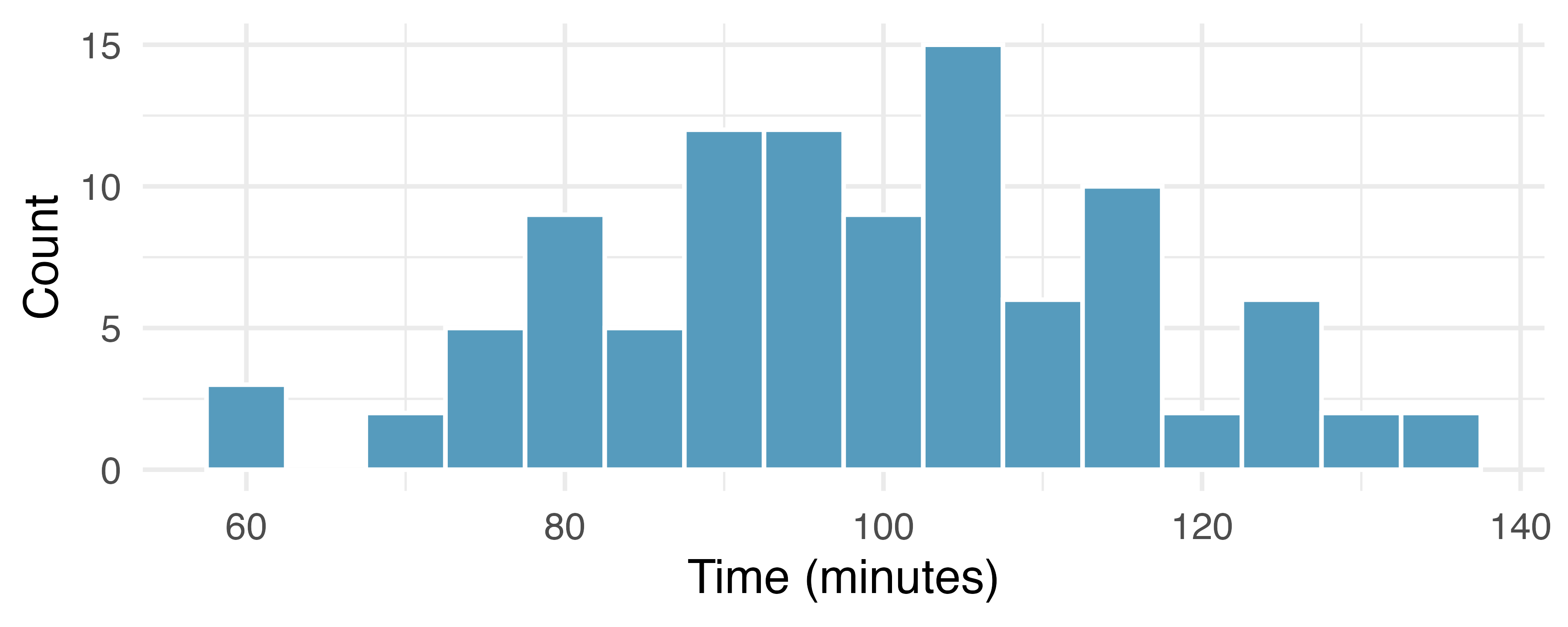
With both the independence and normality conditions satisfied, we can proceed with a hypothesis test using the \(t\)-distribution. The sample mean and sample standard deviation of the sample of 100 runners from the 2017 Cherry Blossom Race are 98.78 and 16.59 minutes, respectively. Recall that the average run time in 2006 was 93.29 minutes. Find the test statistic and p-value. What is your conclusion?
To find the test statistic (T score), we first must determine the standard error:
\[ SE = 16.6 / \sqrt{100} = 1.66 \] Now we can compute the T score using the sample mean (98.78), null value (93.29), and \(SE:\)
\[ T = \frac{98.8 - 93.29}{1.66} = 3.32 \] For \(df = 100 - 1 = 99,\) we can determine using statistical software (or a \(t\)-table) that the one-tail area is 0.000631, which we double to get the p-value: 0.00126.
# use pt() to find the left tail and multiply by 2 to get both tails
(1 - pt(3.32, df = 99)) * 2
[1] 0.00126Because the p-value is smaller than 0.05, we reject the null hypothesis. That is, the data provide convincing evidence that the average run time for the Cherry Blossom Run in 2017 is different than the 2006 average.
When using a \(t\)-distribution, we use a T score (similar to a Z score).
To help us remember to use the \(t\)-distribution, we use a \(T\) to represent the test statistic, and we often call this a T score. The Z score and T score are computed in the exact same way and are conceptually identical: each represents how many standard errors the observed value is from the null value.
19.3 Chapter review
19.3.1 Summary
In this chapter we extended the randomization / bootstrap / mathematical model paradigm to questions involving quantitative variables of interest. When there is only one variable of interest, we are often hypothesizing or finding confidence intervals about the population mean. Note, however, the bootstrap method can be used for other statistics like the population median or the population IQR. When comparing a quantitative variable across two groups, the question often focuses on the difference in population means (or sometimes a paired difference in means). The questions revolving around one, two, and paired samples of means are addressed using the t-distribution; they are therefore called “t-tests” and “t-intervals.” When considering a quantitative variable across 3 or more groups, a method called ANOVA is applied. Again, almost all the research questions can be approached using computational methods (e.g., randomization tests or bootstrapping) or using mathematical models. We continue to emphasize the importance of experimental design in making conclusions about research claims. In particular, recall that variability can come from different sources (e.g., random sampling vs. random allocation, see Figure 2.8).
19.3.2 Terms
The terms introduced in this chapter are presented in Table 19.2. If you’re not sure what some of these terms mean, we recommend you go back in the text and review their definitions. You should be able to easily spot them as bolded text.
| Central Limit Theorem | point estimate | T score single mean |
| degrees of freedom | SD of observations | t-distribution |
| numerical data | SE single mean | t-test |
19.4 Exercises
Answers to odd-numbered exercises can be found in Appendix A.19.
-
Statistics vs. parameters: one mean. Each of the following scenarios were set up to assess an average value. For each one, identify, in words: the statistic and the parameter.
A sample of 25 New Yorkers were asked how much sleep they get per night.
Researchers at two different universities in California collected information on undergraduates’ heights.
-
Statistics vs. parameters: one mean. Each of the following scenarios were set up to assess an average value. For each one, identify, in words: the statistic and the parameter.
Georgianna samples 20 children from a particular city and measures how many years they have each been playing piano.
Traffic police officers (who are regularly exposed to lead from automobile exhaust) had their lead levels measured in their blood.
-
Heights of adults. Researchers studying anthropometry collected body measurements, as well as age, weight, height and gender, for 507 physically active adults. Summary statistics for the distribution of heights (measured in centimeters, cm), along with a histogram, are provided below.11 (Heinz et al. 2003)
Min 147.2 Q1 163.8 Median 170.3 Mean 171.1 Q3 177.8 Max 198.1 SD 9.4 IQR 14.0 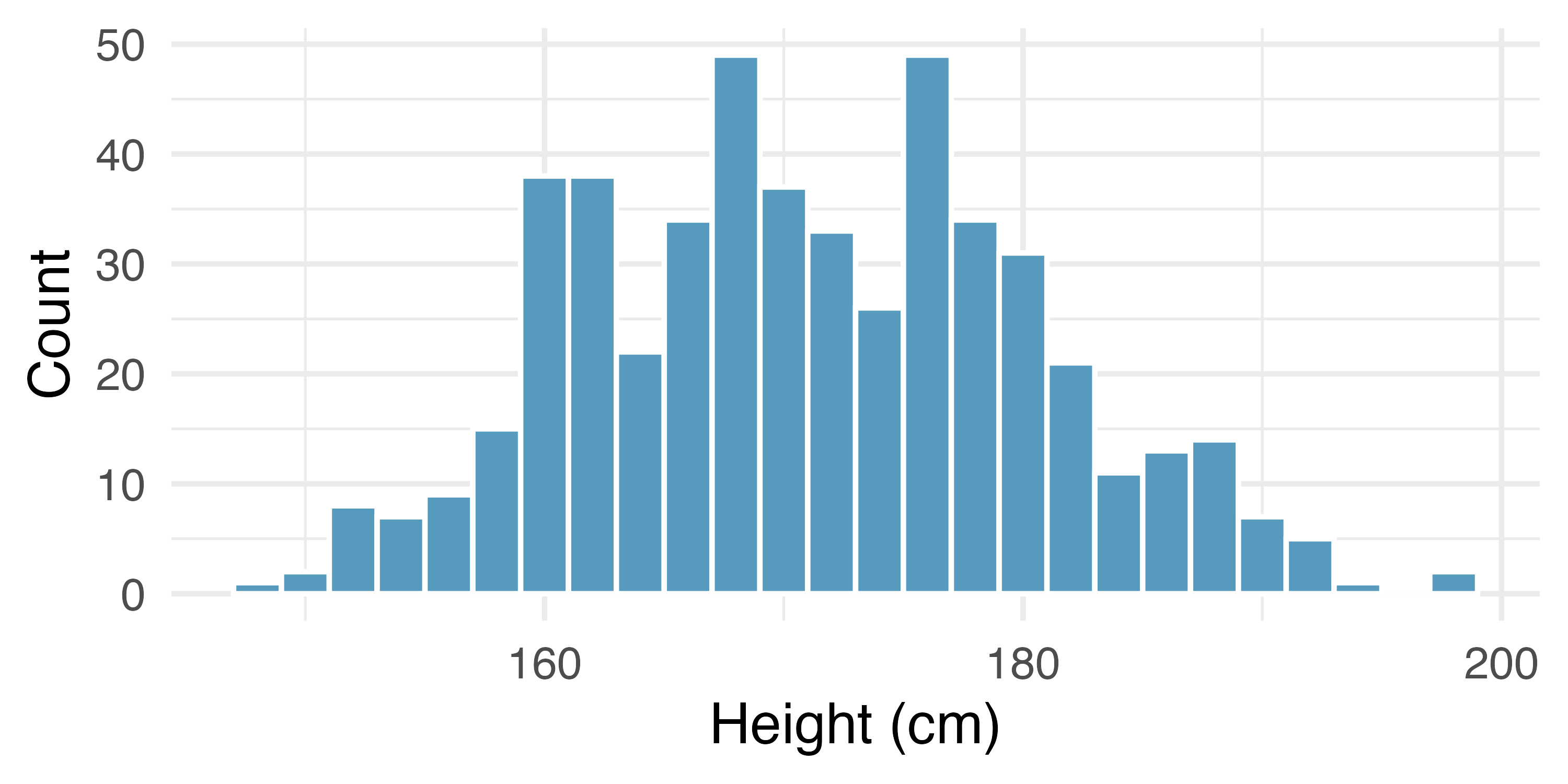
What are the point estimates for the average and median heights of active adults?
What are the point estimates for the standard deviation and IQR of heights of active adults?
Is a person who is 1m 80cm (180 cm) tall considered unusually tall? And is a person who is 1m 55cm (155cm) considered unusually short? Explain your reasoning.
The researchers take another random sample of physically active adults. Would you expect the mean and the standard deviation of this new sample to be the ones given above? Explain your reasoning.
The sample means obtained are point estimates for the mean height of all active individuals, if the sample of individuals is equivalent to a simple random sample. What measure do we use to quantify the variability of such an estimate? Compute this quantity using the data from the original sample under the condition that the data are a simple random sample.
-
Heights of adults, standard error. Heights of 507 physically active adults have a mean of 171 cm and a standard deviation of 9.4 cm. Provide an estimate for the standard error of the mean for samples of following sizes.12 (Heinz et al. 2003)
n = 10
n = 50
n = 100
n = 1000
The standard error of the mean is a number which describes what?
-
Heights of adults vs. kindergartners. Heights of 507 physically active adults have a mean of 171 cm and a standard deviation of 9.4 cm.13 (Heinz et al. 2003)
Would you expect the standard deviation of the heights of a few hundred kindergartners to be higher or lower than 9.4 cm? Explain your reasoning.
Suppose many samples of size 100 adults is taken and, separately, many samples of size 100 kindergarteners are taken. For each of the many samples, the average height is computed. Which set of sample averages would have a larger standard error of the mean, the adult sample averages or the kindergartner sample averages?
-
Heights of adults, bootstrap interval. Researchers studying anthropometry collected body measurements, as well as age, weight, height and gender, for 507 physically active adults. The histogram below shows the sample distribution of bootstrapped means from 1,000 different bootstrap samples.14 (Heinz et al. 2003)
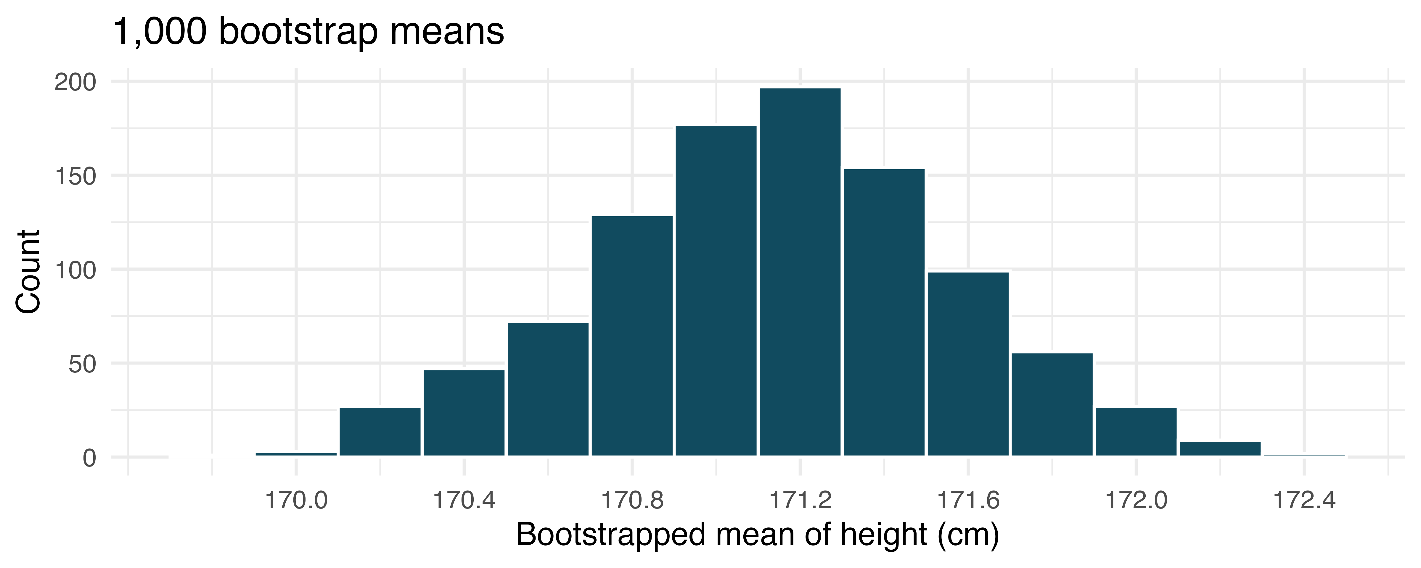
Given the bootstrap sampling distribution for the sample mean, find an approximate value for the standard error of the mean.
By looking at the bootstrap sampling distribution (1,000 bootstrap samples were taken), find an approximate 90% bootstrap percentile confidence interval for the true average adult height in the population from which the data were randomly sampled. Provide the interval as well as a one-sentence interpretation of the interval.
By looking at the bootstrap sampling distribution (1,000 bootstrap samples were taken), find an approximate 90% bootstrap SE confidence interval for the true average adult height in the population from which the data were randomly sampled. Provide the interval as well as a one-sentence interpretation of the interval.
-
Identify the critical \(t\). A random sample is selected from an approximately normal population with unknown standard deviation. Find the degrees of freedom and the critical \(t\)-value (t\(^\star\)) for the given sample size and confidence level.
\(n = 6\), CL = 90%
\(n = 21\), CL = 98%
\(n = 29\), CL = 95%
\(n = 12\), CL = 99%
-
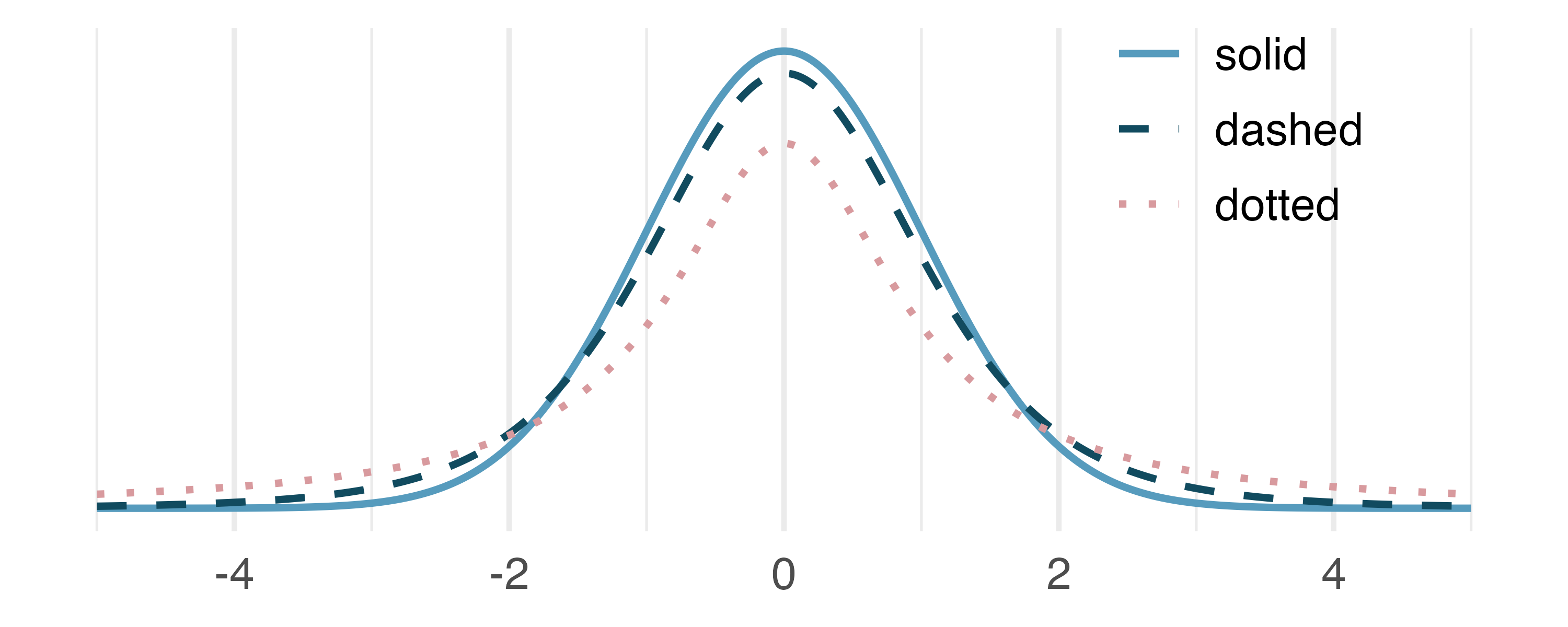
\(t\)-distribution. The figure below shows three unimodal and symmetric curves: the standard normal (z) distribution, the \(t\)-distribution with 5 degrees of freedom, and the \(t\)-distribution with 1 degree of freedom. Determine which is which, and explain your reasoning.
-
Find the p-value, I. A random sample is selected from an approximately normal population with an unknown standard deviation. Find the p-value for the given sample size and test statistic. Also determine if the null hypothesis would be rejected at \(\alpha = 0.05\).
\(n = 11\), \(T = 1.91\)
\(n = 17\), \(T = -3.45\)
\(n = 7\), \(T = 0.83\)
\(n = 28\), \(T = 2.13\)
-
Find the p-value, II. A random sample is selected from an approximately normal population with an unknown standard deviation. Find the p-value for the given sample size and test statistic. Also determine if the null hypothesis would be rejected at \(\alpha = 0.01\).
\(n = 26\), \(T = 2.485\)
\(n = 18\), \(T = 0.5\)
-
Length of gestation, confidence interval. Every year, the United States Department of Health and Human Services releases to the public a large dataset containing information on births recorded in the country. This dataset has been of interest to medical researchers who are studying the relation between habits and practices of expectant mothers and the birth of their children. In this exercise we work with a random sample of 1,000 cases from the dataset released in 2014. The length of pregnancy, measured in weeks, is commonly referred to as gestation. The histograms below show the distribution of lengths of gestation from the random sample of 1,000 births (on the left) and the distribution of bootstrapped means of gestation from 1,500 different bootstrap samples (on the right).15
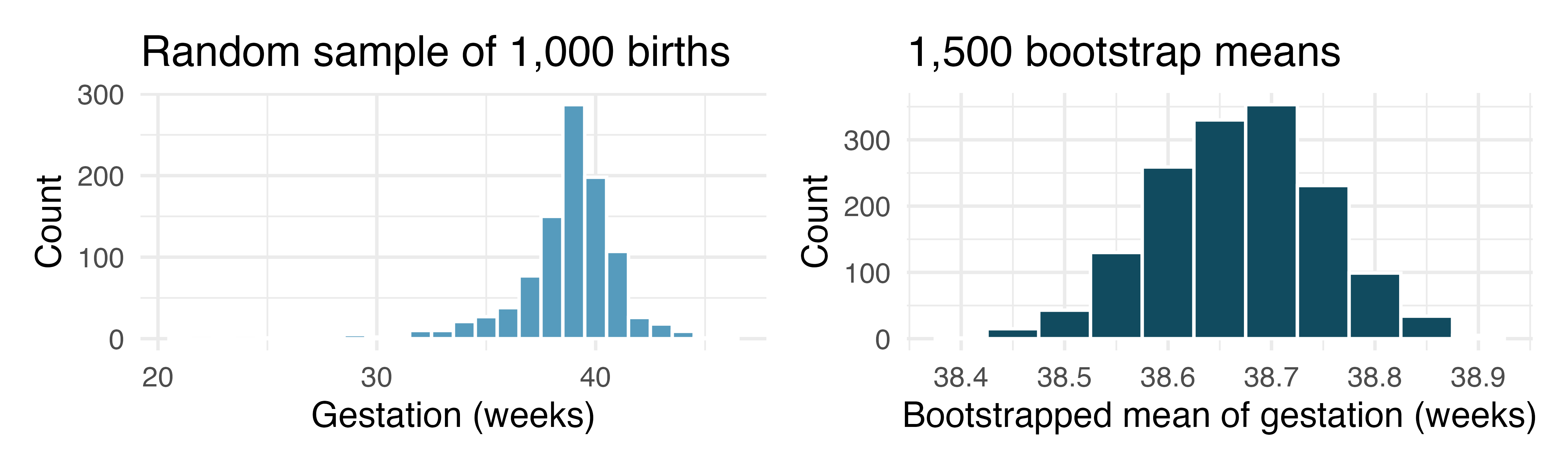
Given the bootstrap sampling distribution for the sample mean, find an approximate value for the standard error of the mean.
By looking at the bootstrap sampling distribution (1,500 bootstrap samples were taken), find an approximate 99% bootstrap percentile confidence interval for the true average gestation length in the population from which the data were randomly sampled. Provide the interval as well as a one-sentence interpretation of the interval.
By looking at the bootstrap sampling distribution (1,500 bootstrap samples were taken), find an approximate 99% bootstrap SE confidence interval for the true average gestation length in the population from which the data were randomly sampled. Provide the interval as well as a one-sentence interpretation of the interval.
-
Length of gestation, hypothesis test. In this exercise we work with a random sample of 1,000 cases from the dataset released by the United States Department of Health and Human Services in 2014. Provided below are sample statistics for gestation (length of pregnancy, measured in weeks) of births in this sample.16
Min Q1 Median Mean Q3 Max SD IQR 21 38 39 38.7 40 46 2.6 2 What is the point estimate for the average length of pregnancy for all women? What about the median?
You might have heard that human gestation is typically 40 weeks. Using the data, perform a complete hypothesis test, using mathematical models, to assess the 40 week claim. State the null and alternative hypotheses, find the T score, find the p-value, and provide a conclusion in context of the data.
A quick internet search validates the claim of “40 weeks gestation” for humans. A friend of yours claims that there are different ways to measure gestation (starting at first day of last period, ovulation, or conception) which will result in estimates that are a week or two different. Another friend mentions that recent increases in cesarean births is likely to have decreased length of gestation. Do the data provide a mechanism to distinguish between your two friends’ claims?
-
Interpreting confidence intervals for population mean. For each of the following statements, indicate if they are a true or false interpretation of the confidence interval. If false, provide a reason or correction to the misinterpretation. You collect a large sample and calculate a 95% confidence interval for the average number of cans of sodas consumed annually per adult in the US to be (440 cans, 520 cans), i.e., on average, adults in the US consume just under two cans of soda per day.
95% of adults in the US consume between 440 and 520 cans of soda per year.
There is a 95% probability that the true population average per adult yearly soda consumption is between 440 and 520 cans.
The true population average per adult yearly soda consumption is between 440 and 520 cans, with 95% confidence.
The average soda consumption of the people who were sampled is between 440 and 520 cans of soda per year, with 95% confidence.
-
Interpreting p-values for population mean. For each of the following statements, indicate if they are a true or false interpretation of the p-value. If false, provide a reason or correction to the misinterpretation. You are wondering if the average amount of cereal in a 10oz cereal box is greater than 10oz. You collect 50 boxes of cereal, weigh them carefully, find a T score, and a p-value of 0.23.
The probability that the average weight of all cereal boxes is 10 oz is 0.23.
The probability that the average weight of all cereal boxes is greater than 10 oz is 0.23.
Because the p-value is 0.23, the average weight of all cereal boxes is 10 oz.
Because the p-value is small, the population average must be just barely above 10 oz.
If \(H_0\) is true, the probability of observing another sample with an average as or more extreme as the data is 0.23.
- Working backwards, I. A 95% confidence interval for a population mean, \(\mu\), is given as (18.985, 21.015). The population distribution is approximately normal and the population standard deviation is unknown. This confidence interval is based on a simple random sample of 36 observations. Assuming that all conditions necessary for inference are satisfied, and using the \(t\)-distribution, calculate the sample mean, the margin of error, and the sample standard deviation.
- Working backwards, II. A 90% confidence interval for a population mean is (65, 77). The population distribution is approximately normal and the population standard deviation is unknown. This confidence interval is based on a simple random sample of 25 observations. Assuming that all conditions necessary for inference are satisfied, and using the \(t\)-distribution, calculate the sample mean, the margin of error, and the sample standard deviation.
-
Sleep habits of New Yorkers. New York is known as “the city that never sleeps”. A random sample of 25 New Yorkers were asked how much sleep they get per night. Statistical summaries of these data are shown below. The point estimate suggests New Yorkers sleep less than 8 hours a night on average. Evaluate the claim that New York is the city that never sleeps keeping in mind that, despite this claim, the true average number of hours New Yorkers sleep could be less than 8 hours or more than 8 hours.
n Mean SD Min Max 25 7.73 0.77 6.17 9.78 Write the hypotheses in symbols and in words.
Check conditions, then calculate the test statistic, \(T\), and the associated degrees of freedom.
Find and interpret the p-value in this context. Drawing a picture may be helpful.
What is the conclusion of the hypothesis test?
If you were to construct a 90% confidence interval that corresponded to this hypothesis test, would you expect 8 hours to be in the interval?
-
Find the mean. You are given the hypotheses shown below. We know that the sample standard deviation is 8 and the sample size is 20. For what sample mean would the p-value be equal to 0.05? Assume that all conditions necessary for inference are satisfied.
\[H_0: \mu = 60 \quad \quad H_A: \mu \neq 60\]
- \(t^\star\) for the correct confidence level. As you’ve seen, the tails of a \(t-\)distribution are longer than the standard normal which results in \(t^{\star}_{df}\) being larger than \(z^{\star}\) for any given confidence level. When finding a CI for a population mean, explain how mistakenly using \(z^{\star}\) (instead of the correct \(t^{*}_{df}\)) would affect the confidence level.
-
Possible bootstrap samples. Consider a simple random sample of the following observations: 47, 4, 92, 47, 12, 8. Which of the following could be a possible bootstrap samples from the observed data above? If the set of values could not be a bootstrap sample, indicate why not.
47, 47, 47, 47, 47, 47
92, 4, 13, 8, 47, 4
92, 47, 12
8, 47, 12, 12, 8, 4, 92
12, 4, 8, 8, 92, 12
-
Play the piano. Georgianna claims that in a small city renowned for its music school, the average child takes less than 5 years of piano lessons. We have a random sample of 20 children from the city, with a mean of 4.6 years of piano lessons and a standard deviation of 2.2 years.
Evaluate Georgianna’s claim (or that the opposite might be true) using a hypothesis test.
Construct a 95% confidence interval for the number of years students in this city take piano lessons, and interpret it in context of the data.
Do your results from the hypothesis test and the confidence interval agree? Explain your reasoning.
-
Auto exhaust and lead exposure. Researchers interested in lead exposure due to car exhaust sampled the blood of 52 police officers subjected to constant inhalation of automobile exhaust fumes while working traffic enforcement in a primarily urban environment. The blood samples of these officers had an average lead concentration of 124.32 \(\mu\)g/l and a SD of 37.74 \(\mu\)g/l; a previous study of individuals from a nearby suburb, with no history of exposure, found an average blood level concentration of 35 \(\mu\)g/l. (Mortada et al. 2000)
Write down the hypotheses that would be appropriate for testing if the police officers appear to have been exposed to a different concentration of lead.
Explicitly state and check all conditions necessary for inference on these data.
Test the hypothesis that the downtown police officers have a higher lead exposure than the group in the previous study. Interpret your results in context.
There is a large literature on understanding and improving bootstrap intervals, see Hesterberg (2015) titled “What Teachers Should Know About the Bootstrap” and Hayden (2019) titled “Questionable Claims for Simple Versions of the Bootstrap” for more information.↩︎
Using the formula for the bootstrap SE interval, we find the 95% confidence interval for \(\mu\) is: \(17,140 \pm 2 \cdot 2,891.87 \rightarrow\) ($11,356.26, $22,923.74). We are 95% confident that the true average car price at Awesome Auto is somewhere between $11,356.26 and $22,923.74.↩︎
Based on the percentile values in Figure 19.6, the middle 90% of the bootstrapped standard deviations is given by the 5th ($3,602.5) and the 95th percentiles ($8,737.2). That is, we are 90% confident that the true standard deviation of car prices is between $3,602.5 and $8,737.2. A 90% confidence level indicates that there was not a need for a high level of confidence, such a 95% or 99%. A lower confidence level has higher potential for error, but it also produces a narrower interval.↩︎
More nuanced guidelines would consider further relaxing the particularly extreme outlier check when the sample size is very large. However, we’ll leave further discussion here to a future course.↩︎
We want to find the shaded area above -1.79 (we leave the picture to you). The lower tail area has an area of 0.0447, so the upper area would have an area of \(1 - 0.0447 = 0.9553.\)↩︎
The sample size is under 30, so we check for obvious outliers: since all observations are within 2 standard deviations of the mean, there are no such clear outliers.↩︎
\(\bar{x} \ \pm\ t^{\star}_{14} \times SE \ \to\ 0.287 \ \pm\ 1.76 \times 0.0178 \ \to\ (0.256, 0.318).\) We are 90% confident that the average mercury content of croaker white fish (Pacific) is between 0.256 and 0.318 ppm.↩︎
No, a confidence interval only provides a range of plausible values for a population parameter, in this case the population mean. It does not describe what we might observe for individual observations.↩︎
\(H_0:\) The average 10-mile run time was the same for 2006 and 2017. \(\mu = 93.29\) minutes. \(H_A:\) The average 10-mile run time for 2017 was different than that of 2006. \(\mu \neq 93.29\) minutes.↩︎
With a sample of 100, we should only be concerned if there is are particularly extreme outliers. The histogram of the data does not show any outliers of concern (and arguably, no outliers at all).↩︎
The
bdimsdata used in this exercise can be found in the openintro R package.↩︎The
bdimsdata used in this exercise can be found in the openintro R package.↩︎The
bdimsdata used in this exercise can be found in the openintro R package.↩︎The
bdimsdata used in this exercise can be found in the openintro R package.↩︎The
births14data used in this exercise can be found in the openintro R package.↩︎The
births14data used in this exercise can be found in the openintro R package.↩︎