English

Appendix A — Exercise solutions

A.1 Chapter 1

23 observations and 7 variables.
(a) “Is there an association between air pollution exposure and preterm births?” (b) 143,196 births in Southern California between 1989 and 1993. (c) Concentrations of carbon monoxide, nitrogen dioxide, ozone, and particulate matter with an aerodynamic diameter of 10 micrometres or less (PM$_{10}$) measured at air quality monitoring stations as well as length of gestation. Continuous numerical variables.
(a) “What is the effect of gamification on learning outcomes compared to traditional teaching methods?” (b) 365 college students taking a statistics course (c) Gender (categorical), level of studies (categorical, ordinal), academic major (categorical), expertise in English language (categorical, ordinal), use of personal computers and games (categorical, ordinal), treatment group (categorical), score (numerical, discrete).
(a) Treatment: $10/43 = 0.23 \rightarrow 23\%$. (b) Control: $2/46 = 0.04 \rightarrow 4\%$. (c) A higher percentage of patients in the treatment group were pain free 24 hours after receiving acupuncture. (d) It is possible that the observed difference between the two group percentages is due to chance. (e) Explanatory: acupuncture or not. Response: if the patient was pain free or not.
(a) Experiment; researchers are evaluating the effect of fines on parents’ behavior related to picking up their children late from daycare. (b) 200 cases: the weekly observations of the 10 daycare centers over the 20 weeks. (c) Number of late pickups (discrete numerical). (d) Week (numerical, discrete), group (categorical, nominal), and study period (categorical, ordinal).
(a) 344 cases (penguins) are included in the data. (b) There are 4 numerical variables in the data: bill length, bill depth, and flipper length (measured in millimeters) and body mass (measured in grams). They are all continuous. (c) There are 3 categorical variables in the data: species (Adelie, Chinstrap, Gentoo), island (Torgersen, Biscoe, and Dream), and sex (female and male).
(a) Airport ownership status (public/private), airport usage status (public/private), region (Central, Eastern, Great Lakes, New England, Northwest Mountain, Southern, Southwest, Western Pacific), latitude, and longitude. (b) Airport ownership status: categorical, not ordinal. Airport usage status: categorical, not ordinal. Region: categorical, not ordinal. Latitude: numerical, continuous. Longitude: numerical, continuous.
(a) Year, number of baby girls named Fiona born in that year, nation. (b) Year (numerical, discrete), number of baby girls named Fiona born in that year (numerical, discrete), nation (categorical, nominal).
(a) County, state, driver’s race, whether the car was searched or not, and whether the driver was arrested or not. (b) All categorical, non-ordinal. (c) Response: whether the car was searched or not. Explanatory: race of the driver.
(a) Observational study. (b) Dog: Lucy. Cat: Luna. (c) Oliver and Lily. (d) Positive, as the popularity of a name for dogs increases, so does the popularity of that name for cats.

A.2 Chapter 2

(a) Population mean, $\mu_{2007} = 52$; sample mean, $\bar{x}_{2008} = 58$. (b) Population mean, $\mu_{2001} = 3.37$; sample mean, $\bar{x}_{2012} = 3.59$.
(a) Population: all births, sample: 143,196 births between 1989 and 1993 in Southern California. (b) If births in this time span at the geography can be considered to be representative of all births, then the results are generalizable to the population of Southern California. However, since the study is observational the findings cannot be used to establish causal relationships.
(a) The population of interest is all college students studying statistics. The sample consists of 365 such students. (b) If the students in this sample, who are likely not randomly sampled, can be considered to be representative of all college students studying statistics, then the results are generalizable to the population defined above. This is probably not a reasonable assumption since these students are from two specific majors only. Additionally, since the study is experimental, the findings can be used to establish causal relationships.
(a) Observation. (b) Variable. (c) Sample statistic (mean). (d) Population parameter (mean).
(a) Observational. (b) Use stratified sampling to randomly sample a fixed number of students, say 10, from each section for a total sample size of 40 students.
(a) Positive, non-linear, somewhat strong. Countries in which a higher percentage of the population have access to the internet also tend to have higher average life expectancies, however rise in life expectancy trails off before around 80 years old. (b) Observational. (c) Wealth: countries with individuals who can widely afford the internet can probably also afford basic medical care. (Note: Answers may vary.)
(a) Simple random sampling is okay. In fact, it’s rare for simple random sampling to not be a reasonable sampling method! (b) The student opinions may vary by field of study, so the stratifying by this variable makes sense and would be reasonable. (c) Students of similar ages are probably going to have more similar opinions, and we want clusters to be diverse with respect to the outcome of interest, so this would not be a good approach. (Additional thought: the clusters in this case may also have very different numbers of people, which can also create unexpected sample sizes.)
(a) The cases are 200 randomly sampled men and women. (b) The response variable is attitude towards a fictional microwave oven. (c) The explanatory variable is dispositional attitude. (d) Yes, the cases are sampled randomly, recruited online using Amazon’s Mechanical Turk. (e) This is an observational study since there is no random assignment to treatments. (f) No, we cannot establish a causal link between the explanatory and response variables since the study is observational. (g) Yes, the results of the study can be generalized to the population at large since the sample is random.
(a) Simple random sample. Non-response bias, if only those people who have strong opinions about the survey responds their sample may not be representative of the population. (b) Convenience sample. Under coverage bias, their sample may not be representative of the population since it consists only of their friends. It is also possible that the study will have non-response bias if some choose to not bring back the survey. (c) Convenience sample. This will have a similar issues to handing out surveys to friends. (d) Multi-stage sampling. If the classes are similar to each other with respect to student composition this approach should not introduce bias, other than potential non-response bias.
(a) Exam performance. (b) Light level: fluorescent overhead lighting, yellow overhead lighting, no overhead lighting (only desk lamps). (c) Wearing glasses or not.
(a) Experiment. (b) Light level (overhead lighting, yellow overhead lighting, no overhead lighting) and noise level (no noise, construction noise, and human chatter noise). (c) Since the researchers want to ensure equal representation of those wearing glasses and not wearing glasses, wearing glasses is a blocking variable.
Need randomization and blinding. One possible outline: (1) Prepare two cups for each participant, one containing regular Coke and the other containing Diet Coke. Make sure the cups ar identical and contain equal amounts of soda. Label the cups (regular) and B (diet). (Be sure to randomize A and B for each trial!) (2) Give each participant the two cups, one cup at a time, in random order, and ask the participant to record a value that indicates ho much she liked the beverage. Be sure that neither the participant nor the person handing out the cups knows the identity of th beverage to make this a double-blind experiment. (Answers may vary.)
(a) Experiment. (b) Treatment: 25 grams of chia seeds twice a day, control: placebo. (c) Yes, gender. (d) Yes, single blind since the patients were blinded to the treatment they received. (e) Since this is an experiment, we can make a causal statement. However, since the sample is not random, the causal statement cannot be generalized to the population at large.
(a) Non-responders may have a different response to this question, e.g., parents who returned the surveys likely don’t have difficulty spending time with their children. (b) It is unlikely that the women who were reached at the same address 3 years later are a random sample. These missing responders are probably renters (as opposed to homeowners) which means that they might have a lower socio-economic status than the respondents. (c) There is no control group in this study, this is an observational study, and there may be confounding variables, e.g., these people may go running because they are generally healthier and/or do other exercises.
(a) Randomized controlled experiment. (b) Explanatory: treatment group (categorical, with 3 levels). Response variable: Psychological well-being. (c) No, because the participants were volunteers. (d) Yes, because it was an experiment. (e) The statement should say “evidence” instead of “proof”.

A.3 Chapter 3

Application chapter, no exercises.

A.4 Chapter 4

(a) We see the order of the categories and the relative frequencies in the bar plot. (b) There are no features that are apparent in the pie chart but not in the bar plot. (c) We usually prefer to use a bar plot as we can also see the relative frequencies of the categories in this graph.
(a) The horizontal locations at which the age groups break into the various opinion levels differ, which indicates that likelihood of supporting protests varies by age group. Two variables may be associated. (b) Answers may vary. Political ideology/leaning and education level.
(a) Number of participants in each group. (b) Proportion of survival. (c) The standardized bar plot should be displayed as a way to visualize the survival improvement in the treatment versus the control group.
(a) The ridge plots do not tell us about the relationship between meat consumption and life expectancy. While it is true that the high income group of countries has highest meat consumption and highest life expectancy, we can’t, for example, differentiate meat consumption across the low and middle income groups (so as to connect to life expectancy). Additionally, we don’t know anything about the relationship betwen meat consumption and life expectancy within an income group. (b) When a relationship is confounded we cannot determine the causal mechanism. We don’t know if the longer life expecancy is due to meat consumption or due to higher income (which comes with many other life-extending practices). (c) In order to investigate a specific confounding variable, first break the data into categories according to that confounding variable (here, income). Then look at the relationship of interest (here meat consumption and life expectancy) separately for each of the levels of the confounding variable (income).
(a) 41% of the JetBlue flights are delayed. 40.7% of the United Airlines flights are delayed. (b) For SFO: JetBlue had 39.7% delayed, United had 40% delayed (United had more delayed flights). For LAX: JetBlue had 40.1% delayed, United had 41% delayed (United had more delayed flights). For BQN: JetBlue had 45.7% delayed, United had 48.8% delayed (United had more delayed flights). (c) Note that JetBlue had substantially more flights than United out of BQN (where there was a high delay percentage). United had substantially more flights than United out of SFO and LAX, both of which had low delay percentages. So JetBlue’s overall percentage delay is bumped up due to the BQN flights, and United’s overall percentage delay is bumped down due to the SFO and LAX flights.

A.5 Chapter 5

(a) Positive association: mammals with longer gestation periods tend to live longer as well. (b) Association would still be positive. (c) No, they are not independent. See part (a).
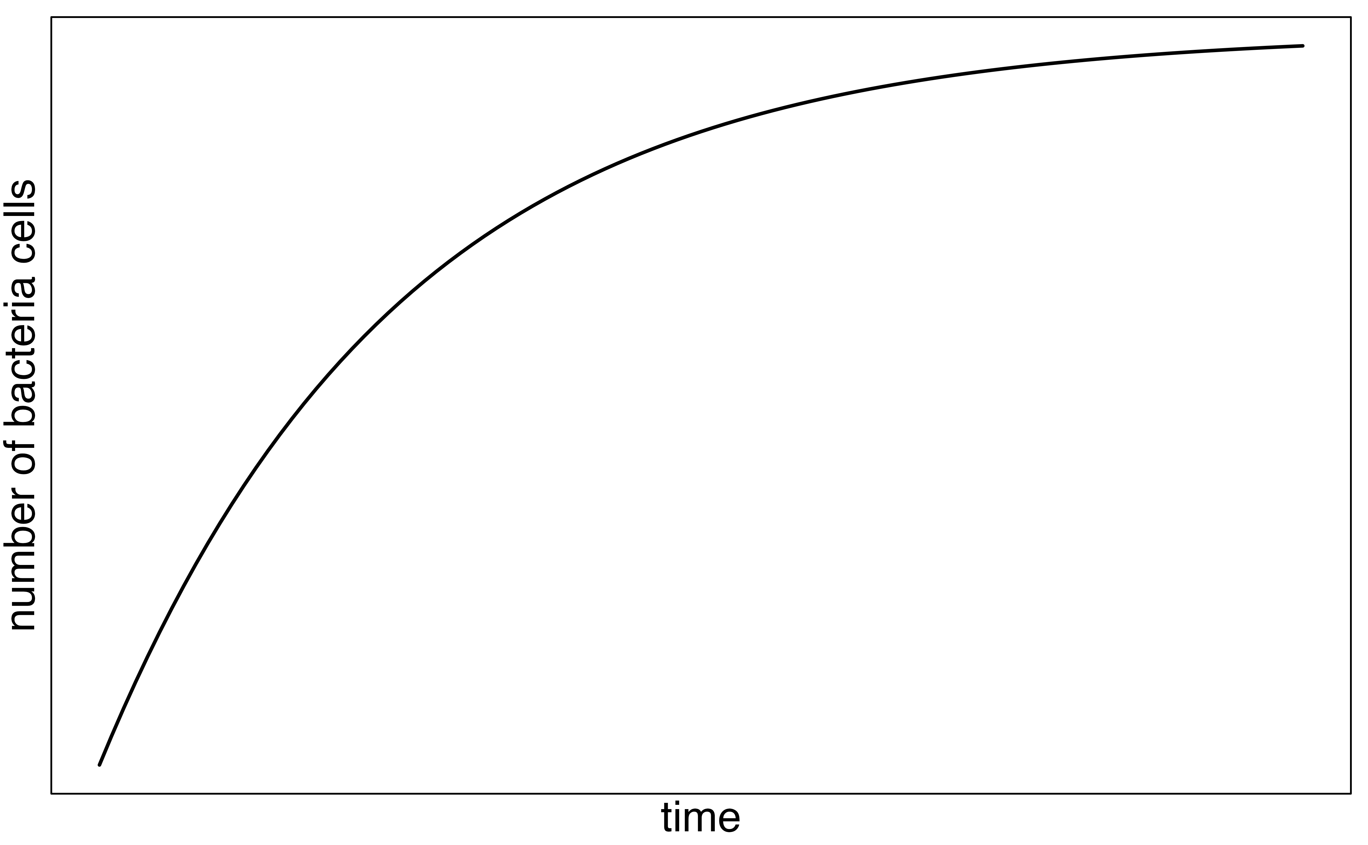
The graph below shows a ramp up period. There may also be a period of exponential growth at the start before the size of the petri dish becomes a factor in slowing growth.
(a) Decrease: the new score is smaller than the mean of the 24 previous scores. (b) Calculate a weighted mean. Use a weight of 24 for the old mean and 1 for the new mean: $(24\times 74 + 1\times64)/(24+1) = 73.6$. (c) The new score is more than 1 standard deviation away from the previous mean, so increase.
Any 10 employees whose average number of days off is between the minimum and the mean number of days off for the entire workforce at this plant.
(a) Dist B has a higher mean since $20 > 13$, and a higher standard deviation since 20 is further from the rest of the data than 13. (b) Dist A has a higher mean since $-20 > -40$, and Dist B has a higher standard deviation since -40 is farther away from the rest of the data than -20. (c) Dist B has a higher mean since all values in this Dist Are higher than those in Dist A, but both distribution have the same standard deviation since they are equally variable around their respective means. (d) Both distributions have the same mean since they’re both centered at 300, but Dist B has a higher standard deviation since the observations are farther from the mean than in Dist A.
(a) About 26. (b) Since the distribution is right skewed the mean is higher than the median. (c) Q1: between 15 and 20, Q3: between 35 and 40, IQR: about 20. (d) Values that are considered to be unusually low or high lie more than 1.5$\times$IQR away from the quartiles. Upper fence: Q3 + 1.5 $\times$ IQR = $37.5 + 1.5 \times 20 = 67.5$; Lower fence: Q1 - 1.5 $\times$ IQR = $17.5 + 1.5 \times 20 = -12.5$; The lowest AQI recorded is not lower than 5 and the highest AQI recorded is not higher than 65, which are both within the fences. Therefore none of the days in this sample would be considered to have an unusually low or high AQI.
The histogram shows that the distribution is bimodal, which is not apparent in the box plot. The box plot makes it easy to identify more precise values of observations outside of the whiskers.
(a) Right skewed, there is a natural boundary at 0 and only a few people have many pets. Center: median, variability: IQR. (b) Right skewed, there is a natural boundary at 0 and only a few people live a very long distance from work. Center: median, variability: IQR. (c) Symmetric. Center: mean, variability: standard deviation. (d) Left skewed. Center: median, variability: IQR. (e) Left skewed. Center: median, variability: IQR.
No, we would expect this distribution to be right skewed. There are two reasons for this: there is a natural boundary at 0 (it is not possible to watch less than 0 hours of TV) and the standard deviation of the distribution is very large compared to the mean.
No, the outliers are likely the maximum and the minimum of the distribution so a statistic based on these values cannot be robust to outliers.
The 75th percentile is 82.5, so 5 students will get an A. Also, by definition 25% of students will be above the 75th percentile.
(a) If $\frac{\bar{x}}{median} = 1$, then $\bar{x} = median$. This is most likely to be the case for symmetric distributions. (b) If $\frac{\bar{x}}{median} < 1$, then $\bar{x} < median$. This is most likely to be the case for left skewed distributions, since the mean is affected (and pulled down) by the lower values more so than the median. (c) If $\frac{\bar{x}}{median} > 1$, then $\bar{x} > median$. This is most likely to be the case for right skewed distributions, since the mean is affected (and pulled up) by the higher values more so than the median.
(a) The distribution of percentage of population that is Hispanic is extremely right skewed with majority of counties with less than 10% Hispanic residents. However there are a few counties that have more than 90% Hispanic population. It might be preferable to, in certain analyses, to use the log-transformed values since this distribution is much less skewed. (b) The map reveals that counties with higher proportions of Hispanic residents are clustered along the Southwest border, all of New Mexico, a large swath of Southwest Texas, the bottom two-thirds of California, and in Southern Florida. In the map all counties with more than 40% of Hispanic residents are indicated by the darker shading, so it is impossible to discern how high Hispanic percentages go. The histogram reveals that there are counties with over 90% Hispanic residents. The histogram is also useful for estimating measures of center and spread. (c) Both visualizations are useful, but if we could only examine one, we should examine the map since it explicitly ties geographic data to each county’s percentage.

A.6 Chapter 6

Application chapter, no exercises.

A.7 Chapter 7

(a) The residual plot will show randomly distributed residuals around 0. The variance is also approximately constant. (b) The residuals will show a fan shape, with higher variability for smaller $x$. There will also be many points on the right above the line. There is trouble with the model being fit here.
(a) Strong relationship, but a straight line would not fit the data. (b) Strong relationship, and a linear fit would be reasonable. (c) Weak relationship, and trying a linear fit would be reasonable. (d) Moderate relationship, but a straight line would not fit the data. (e) Strong relationship, and a linear fit would be reasonable. (f) Weak relationship, and trying a linear fit would be reasonable.
(a) Exam 2 since there is less of a scatter in the plot of course grade versus exam 2. Notice that the relationship between Exam 1 and the course grade appears to be slightly nonlinear. (b) (Answers may vary.) If Exam 2 is cumulative it might be a better indicator of how a student is doing in the class.
(a) $r = -0.7$ $\rightarrow$ (4). (b) $r = 0.45$ $\rightarrow$ (3). (c) $r = 0.06$ $\rightarrow$ (1). (d) $r = 0.92$ $\rightarrow$ (2).
(a) There is a moderate, positive, and linear relationship between shoulder girth and height. (b) Changing the units, even if just for one of the variables, will not change the form, direction or strength of the relationship between the two variables.
(a) There is a somewhat weak, positive, possibly linear relationship between the distance traveled and travel time. There is clustering near the lower left corner that we should take special note of. (b) Changing the units will not change the form, direction or strength of the relationship between the two variables. If longer distances measured in miles are associated with longer travel time measured in minutes, longer distances measured in kilometers will be associated with longer travel time measured in hours. (c) Changing units doesn’t affect correlation: $r = 0.636$.
we can write the amount of meat consumption as an exact linear function of the amount of carbohydrate consumption. (a) $carbs = meat - 3.$ (b) $carbs = meat + 2.$ (c) $carbs = 2 \times meat.$ Since the slopes are positive and these are perfect linear relationships, the correlation will be exactly 1 in all three parts. An alternative way to gain insight into this solution is to create a mock dataset, e.g., 5 countries with meat consumption of 10, 20, 50, 75, and 100 kg per capita, find the related carbohydrate consumption for each mock country, then create a scatterplot.
Correlation: no units. Intercept: cal. Slope: cal/cm.
Over-estimate. Since the residual is calculated as $observed - predicted$, a negative residual means that the predicted value is higher than the observed value.
(a) There is a positive, moderate, linear association between number of calories and amount of carbohydrates. In addition, the amount of carbohydrates is more variable for menu items with higher calories, indicating non-constant variance. There also appear to be two clusters of data: a patch of about a dozen observations in the lower left and a larger patch on the right side. (b) Explanatory: number of calories. Response: amount of carbohydrates (in grams). (c) With a regression line, we can predict the amount of carbohydrates for a given number of calories. This may be useful if only calorie counts for the food items are posted but the amount of carbohydrates in each food item is not readily available. (d) Food menu items with higher predicted protein are predicted with higher variability than those without, suggesting that the model is doing a better job predicting protein amount for food menu items with lower predicted proteins.
(a) First calculate the slope: $b_1 = R\times s_y/s_x = 0.636 \times 113 / 99 = 0.726$. Next, make use of the fact that the regression line passes through the point $(\bar{x},\bar{y})$: $\bar{y} = b_0 + b_1 \times \bar{x}$. Plug in $\bar{x}$, $\bar{y}$, and $b_1$, and solve for $b_0$: 51. Solution: $\widehat{travel~time} = 51 + 0.726 \times distance$. (b) $b_1$: For each additional mile in distance, the model predicts an additional 0.726 minutes in travel time. $b_0$: When the distance travelled is 0 miles, the travel time is expected to be 51 minutes. It does not make sense to have a travel distance of 0 miles in this context. Here, the $y$-intercept serves only to adjust the height of the line and is meaningless by itself. (c) $R^2 = 0.636^2 = 0.40$. About 40% of the variability in travel time is accounted for by the model, i.e., explained by the distance travelled. (d) $\widehat{travel~time} = 51 + 0.726 \times distance = 51 + 0.726 \times 103 \approx 126$ minutes. (Note: we should be cautious in our predictions with this model since we have not yet evaluated whether it is a well-fit model.) (e) $e_i = y_i - \hat{y}_i = 168 - 126 = 42$ minutes. A positive residual means that the model underestimates the travel time. (f) No, this calculation would require extrapolation.
(a) $\widehat{\texttt{poverty}} = 4.60 + 2.05 \times \texttt{unemployment\_rate}.$ (b) The model predicts a poverty rate of 4.60% for counties with 0% unemployment, on average. This is not a meaningful value as no counties have such low unexmployment, it just serves to adjust the height of the regression line. (c) For each additional percentage increase in unemployment rate, poverty rate is predicted to be higher, on average, by 2.05%. (d) Unemployment rate explains 46% of the variability in poverty levels in US counties. (e) $\sqrt{0.46} = 0.678.$
(a) There is an outlier in the bottom right. Since it is far from the center of the data, it is a point with high leverage. It is also an influential point since, without that observation, the regression line would have a very different slope. (b) There is an outlier in the bottom right. Since it is far from the center of the data, it is a point with high leverage. However, it does not appear to be affecting the line much, so it is not an influential point. (c) The observation is in the center of the data (in the x-axis direction), so this point does not have high leverage. This means the point won’t have much effect on the slope of the line and so is not an influential point.
(a) There is a negative, moderate-to-strong, somewhat linear relationship between percent of families who own their home and the percent of the population living in urban areas in 2010. There is one outlier: a state where 100% of the population is urban. The variability in the percent of homeownership also increases as we move from left to right in the plot. (b) The outlier is located in the bottom right corner, horizontally far from the center of the other points, so it is a point with high leverage. It is an influential point since excluding this point from the analysis would greatly affect the slope of the regression line.
(a) True. (b) False, correlation is a measure of the linear association between any two numerical variables.
(a) $r = 0.7 \to (1)$ (b) $r = 0.09 \to (4)$ (c) $r = -0.91 \to (2)$ (d) $r = 0.96 \to (3)$.

A.8 Chapter 8

Annika is right. All variables being highly correlated, including the predictor variables being highly correlated with each other, is not desirable as this would result in multicollinearity.
(a) The association between meat consumption and life expectancy is positive, moderate, and curved. (b) While tempting to say that eating meat may lead to a longer life expectancy, we do not have any sense of why the variables are associated. We are better off thinking that the countries with high meat consumption and high life expectancy are similar in many other ways (e.g., income bracket). (c) Within an income bracket, the relationship between meat consumption and life expectancy is not nearly as strong (as compared to when the data are aggregated into one plot).
No, they shouldn’t include all variables as days_since_start and days_since_race are perfectly correlated with each other. They should only include one of them.
(a) $\widehat{\texttt{weight}} = 7.270 - 0.593 \times \texttt{habit}_\texttt{smoker}$. (b) The estimated body weight of babies born to smoking mothers is 0.593 pounds lower than those who are born to non-smoking mothers. Smoker: $\widehat{\texttt{weight}} = 7.270 - 0.593 \times 1 = 6.68$ pounds. Non-smoker: $\widehat{\texttt{weight}} = 7.270 - 0.593 \times 0 = 7.270$ pounds.
(a) Horror movies. (b) Not necessarily, the change in adjusted $R^2$ is quite small.
(a) $\widehat{\texttt{weight}} = -3.82 + 0.26 \times \texttt{weeks} + 0.02 \times \texttt{mage} + 0.37 \times \texttt{sex}_\texttt{male} + 0.02 \times \texttt{visits} - 0.43 \times \texttt{habit}_\texttt{smoker}.$ (b) $b_{\texttt{weeks}}$: The model predicts a 0.26 pound increase in the birth weight of the baby for each additional week in length of pregnancy, all else held constant. $b_{\texttt{habit}_\texttt{smoker}}$: The model predicts a 0.43 pound decrease in the birth weight of the babies born to smoker mothers compared to non-smokers, all else held constant. (c) Habit might be correlated with one of the other variables in the model, which introduces multicollinearity and complicates model estimation. (d) -0.17~lbs.
Remove gained.
Add weeks.

A.9 Chapter 9

(a) False. The line is fit to predict the probability of success, not the binary outcome. (b) False. Residuals are not used in logistic regression like they are in linear regression because the observed value is always either zero or one (and the predicted value is a probability). The goal of the logistic regression is not to get a perfect prediction (of zero or one), so minimizing residuals is not part of the modeling process. (c) True.
(a) There are a few potential outliers, e.g., on the left in the variable total length, but nothing that will be of serious concern in a dataset this large. (b) When coefficient estimates are sensitive to which variables are included in the model, this typically indicates that some variables are collinear. For example, a possum’s gender may be related to its head length, which would explain why the coefficient for sex changed when we removed the variable. Likewise, a possum’s skull width is likely to be related to its head length and probably even much more closely related than the head length was to gender.
(a) The logistic model relating $\hat{p}$ to the predictors may be written as $\log\left( \frac{\hat{p}}{1 - \hat{p}} \right) = 33.5095 - 1.4207\times \texttt{sex}_{\texttt{male}} - 0.2787 \times \texttt{skull\_w} + 0.5687 \times \texttt{total\_l} - 1.8057 \times \texttt{tail\_l}.$ Only total_l has a positive association with a possum being from Victoria. (b) $\hat{p} = 0.0062$. While the probability is very near zero, we have not run diagnostics on the model. We might also be a little skeptical that the model will remain accurate for a possum found in a US zoo. For example, perhaps the zoo selected a possum with specific characteristics but only looked in one region. On the other hand, it is encouraging that the possum was caught in the wild. (Answers regarding the reliability of the model probability will vary.)
(a) The variable exclaim_subj should be removed, since it’s removal reduces AIC the most (and the resulting model has lower AIC than the None Dropped model). (b) The variable cc should be removed. (c) Removing any variable will increase AIC, so we should not remove any variables from this set.
(a) The AIC is smallest using the variables sex, head_l, skull_w, total_l, and tail_l to predict region (AIC = 83.52), so we would choose that model. (b) If the metric is equivalent across two models with different numbers of variables, we usually want the model with smaller number of variables. Sometimes refered to as Occam’s razor, the simplest explanation is often the one that will generalize most effectively.

A.10 Chapter 10

Application chapter, no exercises.

A.11 Chapter 11

(a) Mean. Each student reports a numerical value: a number of hours. (b) Mean. Each student reports a number, which is a percentage, and we can average over these percentages. (c) Proportion. Each student reports Yes or No, so this is a categorical variable and we use a proportion. (d) Mean. Each student reports a number, which is a percentage like in part (b). (e) Proportion. Each student reports whether s/he expects to get a job, so this is a categorical variable and we use a proportion.
(a) Alternative. (b) Null. (c) Alternative. (d) Alternative. (e) Null. (f) Alternative. (g) Null.
(a) $H_0: \mu = 8$ (On average, New Yorkers sleep 8 hours a night.) $H_A: \mu < 8$ (On average, New Yorkers sleep less than 8 hours a night.) (b) $H_0: \mu = 15$ (The average amount of company time each employee spends not working is 15 minutes for March Madness.) $H_A: \mu > 15$ (The average amount of company time each employee spends not working is greater than 15 minutes for March Madness.)
(a) (i) False. Instead of comparing counts, we should compare percentages of people in each group who suffered cardiovascular problems. (ii) True. (iii) False. Association does not imply causation. We cannot infer a causal relationship based on an observational study. The difference from part (ii) is subtle. (iv) True. (b) Proportion of all patients who had cardiovascular problems: $\frac{7,979}{227,571} \approx 0.035$ (c) The expected number of heart attacks in the Rosiglitazone group, if having cardiovascular problems and treatment were independent, can be calculated as the number of patients in that group multiplied by the overall cardiovascular problem rate in the study: $67,593 * \frac{7,979}{227,571} \approx 2370$. (d) (i) $H_0$: The treatment and cardiovascular problems are independent. They have no relationship, and the difference in incidence rates between the Rosiglitazone and Pioglitazone groups is due to chance. $H_A$: The treatment and cardiovascular problems are not independent. The difference in the incidence rates between the Rosiglitazone and Pioglitazone groups is not due to chance and Rosiglitazone is associated with an increased risk of serious cardiovascular problems. (ii) A higher number of patients with cardiovascular problems than expected under the assumption of independence would provide support for the alternative hypothesis as this would suggest that Rosiglitazone increases the risk of such problems. (iii) In the actual study, we observed 2,593 cardiovascular events in the Rosiglitazone group. In the 100 simulations under the independence model, the simulated differences were never so high, which suggests that the actual results did not come from the independence model. That is, the variables do not appear to be independent, and we reject the independence model in favor of the alternative. The study’s results provide convincing evidence that Rosiglitazone is associated with an increased risk of cardiovascular problems.

A.12 Chapter 12

(a) The statistic is the sample proportion (0.289); the parameter is the population proportion (unknown). (b) $\hat{p}$ and $p$. (c) Bootstrap sample proportion. (d) 0.289. (e) Roughly (0.22, 0.35). (f) We can be 90% confident that between 22% and 35% of all YouTube videos take place outdoors.
With 98% confidence, the true proportion of all US adults (in 2022) who get news from social media sometimes or often is between 0.487 and 0.51.
(a) A or perhaps D. (b) A, B, C, or D. (c) B or C. (d) B. (e) None.
(a) This claim is reasonable, since the entire interval lies above 50%. (b) The value of 70% lies outside of the interval, so we have convincing evidence that the researcher’s conjecture is wrong. (c) A 90% confidence interval will be narrower than a 95% confidence interval. Even without calculating the interval, we can tell that 70% would not fall in the interval, and we would reject the researcher’s conjecture based on a 90% confidence level as well.

A.13 Chapter 13

(a) 0.089 (b) 0.069 (c) 0.589 (d) $P(|Z| > 2) = P(Z < -2) + P(Z > 2)$ 0.046
(a) Verbal: $N(\mu = 151, \sigma = 7)$, Quant: $N(\mu = 153, \sigma = 7.67)$. (b) $Z_{VR} = 1.29$, $Z_{QR} = 0.52$. (c) She scored 1.29 standard deviations above the mean on the Verbal Reasoning section and 0.52 standard deviations above the mean on the Quantitative Reasoning section.

She did better on the Verbal Reasoning section since her Z score on that section was higher. (e)$Perc_{VR} = 0.9007 \approx 90\%$, $Perc_{QR} = 0.6990 \approx 70\%$. (f) $100\% - 90\% = 10\%$ did better than her on VR, and $100\% - 70\% = 30\%$ did better than her on QR. (g) We cannot compare the raw scores since they are on different scales. Comparing her percentile scores is more appropriate when comparing her performance to others. (h) Answer to part (b) would not change as Z scores can be calculated for distributions that are not normal. However, we could not answer parts (d)-(f) since we cannot use the normal probability table to calculate probabilities and percentiles without a normal model.

(a) $Z = 0.84$, which corresponds to approximately 159 on QR. (b) $Z = -0.52$, which corresponds to approximately 147 on VR.
(a) $Z = 1.2$, $P(Z > 1.2) = 0.1151$. (b) $Z= -1.28 \to 70.6\circ$F or colder.
(a) $N(25, 2.78)$. (b) $Z = 1.08$, $P(Z > 1.08) = 0.1401$. (c)The answers are very close because only the units were changed. (The only reason why they differ at all because 28$^\circ$ C is 82.4$^\circ$ F, not precisely 83$^\circ$ F.) (d) Since $IQR = Q3 - Q1$, we first need to find $Q3$ and $Q1$ and take the difference between the two. Remember that $Q3$ is the $75^{th}$ and $Q1$ is the $25^{th}$ percentile of a distribution. Q1 = 23.13, Q3 = 26.86, IQR = 26. 86 - 23.13 = 3.73.
(a) Recall that the general formula is $point~estimate \pm z^{\star} \times SE$. First, identify the three different values. The point estimate is 45%, $z^{\star} = 1.96$ for a 95% confidence level, and $SE = 1.2\%$. Then, plug the values into the formula: $45\% \pm 1.96 \times 1.2\% \quad\to\quad (42.6\%, 47.4\%)$ We are 95% confident that the proportion of US adults who live with one or more chronic conditions is between 42.6% and 47.4%. (b) (i) False. Confidence intervals provide a range of plausible values, and sometimes the truth is missed. A 95% confidence interval “misses” about 5% of the time. (ii) True. Notice that the description focuses on the true population value. (iii) True. If we examine the 95% confidence interval, we can see that 50% is not included in this interval. This means that in a hypothesis test, we would reject the null hypothesis that the proportion is 0.5. (iv) False. The standard error describes the uncertainty in the overall estimate from natural fluctuations due to randomness, not the uncertainty corresponding to individuals’ responses.
A Z score of 0.47 denotes that the sample proportion is 0.47 standard errors greater than the hypothesized value of the population proportion.
(a) Sampling distribution. (b) To know whether the distribution is skewed, we need to know the proportion. We’ve been told the proportion is likely above 5% and below 30%, and the success-failure condition would be satisfied for any of these values. If the population proportion is in this range, the sampling distribution will be symmetric. (c) Standard error. (d) The distribution will tend to be more variable when we have fewer observations per sample.

A.14 Chapter 14

(a) $H_0$: Anti-depressants do not affect the symptoms of Fibromyalgia. $H_A$: Anti-depressants do affect the symptoms of Fibromyalgia (either helping or harming). (b) Concluding that anti-depressants either help or worsen Fibromyalgia symptoms when they actually do neither. (c) Concluding that anti-depressants do not affect Fibromyalgia symptoms when they actually do.
(a) Scenario (i) is higher. Recall that a sample mean based on less data tends to be less accurate and have larger standard errors. (b) Scenario (i) is higher. The higher the confidence level, the higher the corresponding margin of error. (c) They are equal. The sample size does not affect the calculation of the p-value for a given Z score. (d) Scenario (i) is higher. If the null hypothesis is harder to reject (lower $\alpha$), then we are more likely to make a Type II error when the alternative hypothesis is true.
The hypotheses should be about the population proportion ($p$), not the sample proportion. The null hypothesis should have an equal sign. The alternative hypothesis should have a not-equals sign, and it should reference the null value, $p_0 = 0.6$, not the observed sample proportion. The correct way to set up these hypotheses is: $H_0: p = 0.6$ and $H_A: p \neq 0.6$.
Regardless of whether the students were making 95% intervals or 90% intervals, seven students with intervals that miss $\pi$ seems totally reasonable. The students should not be docked for the intervals missing $\pi$.
True. If the sample size gets ever larger, then the standard error will become ever smaller. Eventually, when the sample size is large enough and the standard error is tiny, we can find statistically discernible yet very small differences between the null value and point estimate (assuming they are not exactly equal).

A.15 Chapter 15

Application chapter, no exercises.

A.16 Chapter 16

First, the hypotheses should be about the population proportion ($p$), not the sample proportion. Second, the null value should be what we are testing (0.25), not the observed value (0.29). The correct way to set up these hypotheses is: $H_0: p = 0.25$ and $H_A: p > 0.25.$
(a) $H_0 : p = 0.20,$ $H_A : p > 0.20.$ (b) $\hat{p} = 159/650 = 0.245.$ (c) Answers will vary. Each student can be represented with a card. Take 100 cards, 20 black cards representing those who support proposals to defund police departments and 80 red cards representing those who do not. Shuffle the cards and draw with replacement (shuffling each time in between draws) 650 cards representing the 650 respondents to the poll. Calculate the proportion of black cards in this sample, $\hat{p}_{sim},$ i.e., the proportion of those who upport proposals to defund police departments. The p-value will be the proportion of simulations where $\hat{p}_{sim} \geq 0.245.$ (Note: We would generally use a computer to perform the simulations.) (d) There 1 only one simulated proportion that is at least 0.245, therefore the approximate p-value is 0.001. Your p-value may vary slightly since it is based on a visual estimate. Since the p-value is smaller than 0.05, we reject $H_0.$ The data provide convincing evidence that the proportion of Seattle adults who support proposals to defund police departments is greater than 0.20, i.e., more than one in five.
(a) $H_0: p = 0.5$, $H_A: p \ne 0.5$. (b) The p-value is roughly 0.4, There is not evidence in the data (possibly because there are only 7 cats being measured!) to conclude that the cats have a preference one way or the other between the two shapes.
(a) $SE(\hat{p}) = 0.189$. (c) Roughly 0.188. (c) Yes. (d) No. (e) The draws from the null hypothesis are discrete (only a few distinct options) and the mathematical model is continuous (infinite options on a continuum).
(a) The null hypothesis simulation was done with $p=0.7$, and the data bootstrap simulation was done with $p = 0.6.$ (b) The null hypothesis simulation is centered at 0.7; the data bootstrap is centered at 0.6. (c) The standard error of the sample proportion is given to be roughly 0.1 for both histograms. (d) Both histograms are reasonably symmetric. Note that histograms which describe the variability of proportions become more skewed as the center of the distribution gets closer to 1 (or zero) because the boundary of 1.0 restricts the symmetry of the tail of the distribution. For this reason, the null hypothesis simulation histogram is slightly more skewed (left).
(a) The null hypothesis simulation distribution for testing. The data bootstrap distribution for confidence intervals. (b) $H_0: p = 0.7;$ $H_A: p \ne 0.7.$ p-value $> 0.05.$ There is no evidence that the proportion of full-time statistics majors who work is different from 70%. (c) We are 98% confident that the true proportion of all full-time student statistics majors who work at least 5 hours per week is between 35% and 80%. (d) Using $z^\star = 2.33$, the 98% confidence interval is 0.367 to 0.833.
(a) False. Doesn’t satisfy success-failure condition. (b) True. The success-failure condition is not satisfied. In most samples we would expect $\hat{p}$ to be close to 0.08, the true population proportion. While $\hat{p}$ can be much above 0.08, it is bound below by 0, suggesting it would take on a right skewed shape. Plotting the sampling distribution would confirm this suspicion. (c) False. $SE_{\hat{p}} = 0.0243$, and $\hat{p} = 0.12$ is only $\frac{0.12 - 0.08}{0.0243} = 1.65$ SEs away from the mean, which would not be considered unusual. (d) True. $\hat{p}=0.12$ is 2.32 standard errors away from the mean, which is often considered unusual. (e) False. Decreases the SE by a factor of $1/\sqrt{2}$.
(a) True. See the reasoning of 6.1(b). (b) True. We take the square root of the sample size in the SE formula. (c) True. The independence and success-failure conditions are satisfied. (d) True. The independence and success-failure conditions are satisfied.
(a) False. A confidence interval is constructed to estimate the population proportion, not the sample proportion. (b) True. 95% CI: $82\%\ \pm\ 2\%$. (c) True. By the definition of the confidence level. (d) True. Quadrupling the sample size decreases the SE and ME by a factor of $1/\sqrt{4}$. (e) True. The 95% CI is entirely above 50%.
With a random sample, independence is satisfied. The success-failure condition is also satisfied. $ME = z^{\star} \sqrt{ \frac{\hat{p} (1-\hat{p})} {n} } = 1.96 \sqrt{ \frac{0.56 \times 0.44}{600} }= 0.0397 \approx 4\%.$
(a) No. The sample only represents students who took the SAT, and this was also an online survey. (b) (0.5289, 0.5711). We are 90% confident that 53% to 57% of high school seniors who took the SAT are fairly certain that they will participate in a study abroad program in college. (c) 90% of such random samples would produce a 90% confidence interval that includes the true proportion. (d) Yes. The interval lies entirely above 50%.
(a) We want to check for a majority (or minority), so we use the following hypotheses: $H_0: p = 0.5$ and $H_A: p \neq 0.5$. We have a sample proportion of $\hat{p} = 0.55$ and a sample size of $n = 617$ independents. Since this is a random sample, independence is satisfied. The success-failure condition is also satisfied: $617 \times 0.5$ and $617 \times (1 - 0.5)$ are both at least 10 (we use the null proportion $p_0 = 0.5$ for this check in a one-proportion hypothesis test). Therefore, we can model $\hat{p}$ using a normal distribution with a standard error of $SE = \sqrt{\frac{p(1 - p)}{n}} = 0.02$. (We use the null proportion $p_0 = 0.5$ to compute the standard error for a one-proportion hypothesis test.) Next, we compute the test statistic: $Z = \frac{0.55 - 0.5}{0.02} = 2.5.$ This yields a one-tail area of 0.0062, and a p-value of $2 \times 0.0062 = 0.0124.$ Because the p-value is smaller than 0.05, we reject the null hypothesis. We have strong evidence that the support is different from 0.5, and since the data provide a point estimate above 0.5, we have strong evidence to support this claim by the TV pundit. (b) No. Generally we expect a hypothesis test and a confidence interval to align, so we would expect the confidence interval to show a range of plausible values entirely above 0.5. However, if the confidence level is misaligned (e.g., a 99% confidence level and a $\alpha = 0.05$ discernibility level), then this is no longer generally true.
(a) $H_0: p = 0.5$. $H_A: p > 0.5$. Independence (random sample, $<10\%$ of population) is satisfied, as is the success-failure conditions (using $p_0 = 0.5$, we expect 40 successes and 40 failures). $Z = 2.91$ $\to$ p- value $= 0.0018$. Since the p-value $< 0.05$, we reject the null hypothesis. The data provide strong evidence that the rate of correctly identifying a soda for these people is discernibly better than just by random guessing. (b) If in fact people cannot tell the difference between diet and regular soda and they randomly guess, the probability of getting a random sample of 80 people where 53 or more identify a soda correctly would be 0.0018.
(a) The sample is from all computer chips manufactured at the factory during the week of production. We might be tempted to generalize the population to represent all weeks, but we should exercise caution here since the rate of defects may change over time. (b) The fraction of computer chips manufactured at the factory during the week of production that had defects. (c) Estimate the parameter using the data: $\hat{p} = \frac{27}{212} = 0.127$. (d) Standard error (or $SE$). (e) Compute the $SE$ using $\hat{p} = 0.127$ in place of $p$: $SE \approx \sqrt{\frac{\hat{p}(1 - \hat{p})}{n}} = \sqrt{\frac{0.127(1 - 0.127)}{212}} = 0.023$. (f) The standard error is the standard deviation of $\hat{p}$. A value of 0.10 would be about one standard error away from the observed value, which would not represent a very uncommon deviation. (Usually beyond about 2 standard errors is a good rule of thumb.) The engineer should not be surprised. (g) Recomputed standard error using $p = 0.1$: $SE = \sqrt{\frac{0.1(1 - 0.1)}{212}} = 0.021$. This value isn’t very different, which is typical when the standard error is computed using relatively similar proportions (and even sometimes when those proportions are quite different!).
(a) The visitors are from a simple random sample, so independence is satisfied. The success-failure condition is also satisfied, with both 64 and $752 - 64 = 688$ above 10. Therefore, we can use a normal distribution to model $\hat{p}$ and construct a confidence interval. (b) The sample proportion is $\hat{p} = \frac{64}{752} = 0.085$. The standard error is $SE = \sqrt{\frac{0.085 (1 - 0.085)}{752}} = 0.010.$ (c) For a 90% confidence interval, use $z^{\star} = 1.65$. The confidence interval is $0.085 \pm 1.65 \times 0.010 \to (0.0685, 0.1015)$. We are 90% confident that 6.85% to 10.15% of first-time site visitors will register using the new design.

A.17 Chapter 17

(a) The parameter is $p_{Asican-Indian} - p_{Chinese}.$ The statistic is $\hat{p}_{Asian-Indian} - \hat{p}_{Chinese} = 223/4373 - 279/4736 = -0.008$ (b) Roughly 0.005. (c) $H_0: p_{Asian-Indian} - p_{Chinese} = 0;$, $H_A: p_{Asian-Indian} - p_{Chinese} \ne 0.$ The evidence is borderline but worth further study. There is not strong evidence that the true difference in proportion of current smokers is different across the two ethnic groups.
(a) Roughly 0.00625. (b) We are 95% confident that the true proportion of Filipino Americans who are current smokers is between 5.28 and 7.72 percentage points higher in the control vaccine group than the proportion of Chinese Americans who smoke. (c) We are 95% confident that the true proportion of Filipino Americans who are current smokers is between 5.2 and 7.7 percentage points higher in the control vaccine group than the proportion of Chinese Americans who smoke.
(a) While the standard errors of the difference in proportion across the two graphs are roughly the same (approximately 0.012), the centers are not. Computational method A is centered at 0.07 (the difference in the observed sample proportions) and Computational method B is centered at 0. (b) What is the difference between the proportions of Bachelor’s and Associate’s students who believe that the COVID-19 pandemic will negatively impact their ability to complete the degree? (c) Is the proportion of Bachelor’s students who believe that their ability to complete the degree will be negatively impacted by the COVID-19 pandemic different than that of Associate’s students?
(a) 26 Yes and 94 No in Nevaripine and 10 Yes and 110 No in Lopinavir group. (b) $H_0: p_N = p_L$. There is no difference in virologic failure rates between the Nevaripine and Lopinavir groups. $H_A: p_N \ne p_L$. There is some difference in virologic failure rates between the Nevaripine and Lopinavir groups. (c) Random assignment was used, so the observations in each group are independent. If the patients in the study are representative of those in the general population (something impossible to check with the given information), then we can also confidently generalize the findings to the population. The success-failure condition, which we would check using the pooled proportion ($\hat{p}_{pool} = 36/240 = 0.15$), is satisfied. $Z = 2.89$ $\to$ p-value $=0.0039$. Since the p-value is low, we reject $H_0$. There is strong evidence of a difference in virologic failure rates between the Nevaripine and Lopinavir groups. Treatment and virologic failure do not appear to be independent.
(a) Standard error: $SE = \sqrt{\frac{0.79(1 - 0.79)}{347} + \frac{0.55(1 - 0.55)}{617}} = 0.03.$ Using $z^{\star} = 1.96$, we get: $0.79 - 0.55 \pm 1.96 \times 0.03 \to (0.181, 0.299).$ We are 95% confident that the proportion of Democrats who support the plan is 18.1% to 29.9% higher than the proportion of Independents who support the plan. (b) True.
(a) In effect, we’re checking whether men are paid more than women (or vice-versa), and we’d expect these outcomes with either chance under the null hypothesis: $H_0: p = 0.5$ and $H_A: p \neq 0.5.$ We’ll use $p$ to represent the fraction of cases where men are paid more than women. (b) There isn’t a good way to check independence here since the jobs are not a simple random sample. However, independence doesn’t seem unreasonable, since the individuals in each job are different from each other. The success-failure condition is met since we check it using the null proportion: $p_0 n = (1 - p_0) n = 10.5$ is greater than 10. We can compute the sample proportion, $SE$, and test statistic: $\hat{p} = 19 / 21 = 0.905$ and $SE = \sqrt{\frac{0.5 \times (1 - 0.5)}{21}} = 0.109$ and $Z = \frac{0.905 - 0.5}{0.109} = 3.72.$ The test statistic $Z$ corresponds to an upper tail area of about 0.0001, so the p-value is 2 times this value: 0.0002. Because the p-value is smaller than 0.05, we reject the notion that all these gender pay disparities are due to chance. Because we observe that men are paid more in a higher proportion of cases and we have rejected $H_0$, we can conclude that men are being paid higher amounts in ways not explainable by chance alone. If you’re curious for more info around this topic, including a discussion about adjusting for additional factors that affect pay, please see the following video by Healthcare Triage: youtu.be/aVhgKSULNQA.
Before we can calculate a confidence interval, we must first check that the conditions are met. There aren’t at least 10 successes and 10 failures in each of the four groups (treatment/control and yawn/not yawn), $(\hat{p}_C - \hat{p}_T)$ is not expected to be approximately normal and therefore cannot calculate a confidence interval for the difference between the proportions of participants who yawned in the treatment and control groups using large sample techniques and a critical Z score.
(a) False. The confidence interval includes 0. (b) False. We are 95% confident that 16% fewer to 2% Americans who make less than $40,000 per year are not at all personally affected by the government shutdown compared to those who make $40,000 or more per year. (c) False. As the confidence level decreases the width of the confidence level decreases as well. (d) True.
(a) Type I. (b) Type II. (c) Type II.
No. The samples at the beginning and at the end of the semester are not independent since the survey is conducted on the same students.
(a) The proportion of the normal curve centered at -0.1 with a standard deviation of 0.15 that is less than -2 * standard error is 0.09. (b) The proportion of the normal curve centered at -0.4 with a standard deviation of 0.145 that is less than 2 * standard error is 0.78. (c) The proportion of the normal curve centered at -0.1 with a standard deviation of 0.0671 that is less than 2 * standard error is 0.31. (d) The proportion of the normal curve centered at -0.4 with a standard deviation of 0.0678 that is less than 2 * standard error is 1. (e) The larger the value of $\delta$ and the larger the sample size, the more likely that the future study will lead to sample proportions which are able to reject the null hypothesis.

A.18 Chapter 18

(a) Two-way table is shown below. (b-i) $E_{row_1, col_1} = \frac{(row~1~total)\times(col~1~total)}{table~total} = 35$. This is lower than the observed value. (b-ii) $E_{row_2, col_2} = \frac{(row~2~total)\times(col~2~total)}{table~total} = 115$. This is lower than the observed value.

Quit

Treatment Yes No Total

Patch + support group 40 110 150

Only patch 30 120 150

Total 70 230 300
(a) Sun = 0.343, Partial = 0.325, Shade = 0.331. (b) For each, the numbers are listed in the order sun, partial, and shade: Desert (40,9, 38,7, 39.4), Mountain (36.7, 34.8, 35.5), Valley (36.4, 34.5, 35.1). (c) Yes. (d) We can’t evaluate the association without a formal test.
The original dataset will have a higher Chi-squared statistic than the randomized dataset.
(a) The two variables are independent. (b) The randomized Chi-squared values range from zero to approximately 15. (c) The null hypothesis is that the variables are independent; the alternative hypothesis is that the variables are associated. The p-value is extremely small. The habitat provides information about the likelihood of being in the different sunshine states.
(a) The two variables are independent. (b) The randomized Chi-squared values range from zero to approximately 25. (c) The null hypothesis is that the variables are independent; the alternative hypothesis is that the variables are associated. The p-value is around 0. There is convincing evidence to claim that site and sunlight preference are associated. (d) With larger sample sizes, the power (the probability of rejecting $H_0$ when $H_A$ is true) is higher.
(a) False. The Chi-square distribution has one parameter called degrees of freedom. (b) True. (c) True. (d) False. As the degrees of freedom increases, the shape of the Chi-square distribution becomes more symmetric.
The hypotheses are $H_0:$ Sleep levels and profession are independent. $H_A:$ Sleep levels and profession are associated. The observations are independent and the sample sizes are large enough to conduct a Chi-square test of independence. The Chi-square statistic is 1 with 2 degrees of freedom. The p-value is 0.6. Since the p-value is high (default to alpha = 0.05), we fail to reject $H_0$. The data do not provide convincing evidence of an association between sleep levels and profession.
(a) $H_0$: The age of Los Angeles residents is independent of shipping carrier preference variable. $H_A$: The age of Los Angeles residents is associated with the shipping carrier preference variable. (b) The conditions are not satisfied since some expected counts are below 5.

	Quit
Patch + support group	40	110	150
Only patch	30	120	150
Total	70	230	300

A.19 Chapter 19

(a) Average sleep of 25 in sample vs. all New Yorkers. (b) Average height of students in study vs all undergraduates.
(a) Use the sample mean to estimate the population mean: 171.1. Likewise, use the sample median to estimate the population median: 170.3. (b) Use the sample standard deviation (9.4) and sample IQR ($177.8-163.8 = 14$). (c) $Z_{180} = 0.95$ and $Z_{155} = -1.71.$ Neither of these observations is more than two standard deviations away from the mean, so neither would be considered unusual. (d) No, sample point estimates only estimate the population parameter, and they vary from one sample to another. Therefore we cannot expect to get the same mean and standard deviation with each random sample. (e) We use the standard error of the mean to measure the variability in means of random samples of same size taken from a population. The variability in the means of random samples is quantified by the standard error. Based on this sample, $SE_{\bar{x}} = \frac{9.4}{\sqrt{507}} = 0.417.$
(a) The kindergartners will have a smaller standard deviation of heights. We would expect their heights to be more similar to each other compared to a group of adults’ heights. (b) The standard error of the mean will depend on the variability of individual heights. The standard error of the adult sample averages will be around 9.4/$\sqrt{100}$ = 0.94cm. The standard error of the kindergartner sample averages will be smaller.
(a) $df=6-1=5$, $t_{5}^{\star} = 2.02$. (b) $df=21-1=20$, $t_{20}^{\star} = 2.53$. (c) $df=28$, $t_{28}^{\star} = 2.05$. (d) $df=11$, $t_{11}^{\star} = 3.11$.
(a) 0.085, do not reject $H_0$. (b) 0.003, reject $H_0$. (c) 0.438, do not reject $H_0$. (d) 0.042, reject $H_0$.
(a) Roughly 0.1 weeks. (b) Roughly (38.45 weeks, 38.85 weeks). (c) Roughly (38.49 weeks, 38.91 weeks).
(a) False (b) False. (c) True. (d) False.
The mean is the midpoint: $\bar{x} = 20$. Identify the margin of error: $ME = 1.015$, then use $t^{\star}_{35} = 2.03$ and $SE = s/ \sqrt{n}$ in the formula for margin of error to identify $s = 3$.
(a) $H_0$: $\mu = 8$ (New Yorkers sleep 8 hrs per night on average.) $H_A$: $\mu \neq 8$ (New Yorkers sleep less or more than 8 hrs per night on average.) (b) Independence: The sample is random. The min/max suggest there are no concerning outliers. $T = -1.75$. $df=25-1=24$. (c) p-value $= 0.093$. If in fact the true population mean of the amount New Yorkers sleep per night was 8 hours, the probability of getting a random sample of 25 New Yorkers where the average amount of sleep is 7.73 hours per night or less (or 8.27 hours or more) is 0.093. (d) Since p-value $>$ 0.05, do not reject $H_0$. The data do not provide strong evidence that New Yorkers sleep more or less than 8 hours per night on average. (e) Yes, since we did not rejected $H_0$.
With a larger critical value, the confidence interval ends up being wider. This makes intuitive sense as when we have a small sample size and the population standard deviation is unknown, we should have a wider interval than if we knew the population standard deviation, or if we had a large enough sample size.
(a) We will conduct a 1-sample $t$-test. $H_0$: $\mu = 5$. $H_A$: $\mu \neq 5$. We’ll use $\alpha = 0.05$. This is a random sample, so the observations are independent. To proceed, we assume the distribution of years of piano lessons is approximately normal. $SE = 2.2 / \sqrt{20} = 0.4919$. The test statistic is $T = (4.6 - 5) / SE = -0.81$. $df = 20 - 1 = 19$. The one-tail area is about 0.21, so the p-value is about 0.42, which is bigger than $\alpha = 0.05$ and we do not reject $H_0$. That is, we do not have sufficiently strong evidence to reject the notion that the average is 5 years. (b) Using $SE = 0.4919$ and $t_{df = 19}^{\star} = 2.093$, the confidence interval is (3.57, 5.63). We are 95% confident that the average number of years a child takes piano lessons in this city is 3.57 to 5.63 years. (c) They agree, since we did not reject the null hypothesis and the null value of 5 was in the $t$-interval.

A.20 Chapter 20

The hypotheses should use population means ($\mu$) not sample means ($\bar{x}$), the null hypothesis should set the two population means equal to each other, the alternative hypothesis should be two-tailed and use a not equal to sign.
$H_0: \mu_{0.99} = \mu_{1}$ and $H_A: \mu_{0.99} \ne \mu_{1}.$ p-value $<$ 0.05, reject $H_0.$ The data provide convincing evidence that the difference in population averages of price per carat of 0.99 carats and 1 carat diamonds are different.
(a) We are 95% confident that the population average price per carat of 0.99 carat diamonds is $2 to $23 lower than the population average price per carat of 1 carat diamonds. (b) We are 95% confident that the population average price per carat of 0.99 carat diamonds is $2.91 to $21.10 lower than the population average price per carat of 1 carat diamonds.
The difference is not zero (statistically discernible), but there is no evidence that the difference is large (practically important), because the interval provides values as low as 1 lb.
$H_0: \mu_{0.99} = \mu_{1}$ and $H_A: \mu_{0.99} \ne \mu_{1}$. Independence: Both samples are random and represent less than 10% of their respective populations. Also, we have no reason to think that the 0.99 carats are not independent of the 1 carat diamonds since they are both sampled randomly. Normality: The distributions are not extremely skewed, hence we can assume that the distribution of the average differences will be nearly normal as well. $T_{22} = -2.7$, p-value = 0.0131. Since p-value less than 0.05, reject $H_0$. The data provide convincing evidence that the difference in population averages of price per carat of 0.99 carats and 1 carat diamonds are different.
We are 95% confident that the population average price per carat of 0.99 carat diamonds is $2.96 to $22.42 lower than the population average price per carat of 1 carat diamonds.
(a) $\mu_{\bar{x}_1} = 15$, $\sigma_{\bar{x}_1} = 20 / \sqrt{50} = 2.8284.$ (b) $\mu_{\bar{x}_2} = 20$, $\sigma_{\bar{x}_1} = 10 / \sqrt{30} = 1.8257.$ (c) $\mu_{\bar{x}_2 - \bar{x}_1} = 20 - 15 = 5$, $\sigma_{\bar{x}_2 - \bar{x}_1} = \sqrt{\left(20 / \sqrt{50}\right)^2 + \left(10 / \sqrt{30}\right)^2} = 3.3665.$ (d) Think of $\bar{x}_1$ and $\bar{x}_2$ as being random variables, and we are considering the standard deviation of the difference of these two random variables, so we square each standard deviation, add them together, and then take the square root of the sum: $SD_{\bar{x}_2 - \bar{x}_1} = \sqrt{SD_{\bar{x}_2}^2 + SD_{\bar{x}_1}^2}.$
(a) Chicken fed linseed weighed an average of 218.75 grams while those fed horsebean weighed an average of 160.20 grams. Both distributions are relatively symmetric with no apparent outliers. There is more variability in the weights of chicken fed linseed. (b) $H_0: \mu_{ls} = \mu_{hb}$. $H_A: \mu_{ls} \ne \mu_{hb}$. We leave the conditions to you to consider. $T=3.02$, $df = min(11, 9) = 9$ $\to$ p-value $= 0.014$. Since p-value $<$ 0.05, reject $H_0$. The data provide strong evidence that there is a discernible difference between the average weights of chickens that were fed linseed and horsebean. (c) Type I error, since we rejected $H_0$. (d) Yes, since p-value $>$ 0.01, we would not have rejected $H_0$.
$H_0: \mu_C = \mu_S$. $H_A: \mu_C \ne \mu_S$. $T = 3.27$, $df=11$ $\to$ p-value $= 0.007$. Since p-value $< 0.05$, reject $H_0$. The data provide strong evidence that the average weight of chickens that were fed casein is different than the average weight of chickens that were fed soybean (with weights from casein being higher). Since this is a randomized experiment, the observed difference can be attributed to the diet.
$H_0: \mu_{T} = \mu_{C}$. $H_A: \mu_{T} \ne \mu_{C}$. $T=2.24$, $df=21$ $\to$ p-value $= 0.036$. Since p-value $<$ 0.05, reject $H_0$. The data provide strong evidence that the average food consumption by the patients in the treatment and control groups are different. Furthermore, the data indicate patients in the distracted eating (treatment) group consume more food than patients in the control group.

A.21 Chapter 21

Paired, data are recorded in the same cities at two different time points. The temperature in a city at one point is not independent of the temperature in the same city at another time point
(a) Since it’s the same students at the beginning and the end of the semester, there is a pairing between the datasets, for a given student their beginning and end of semester grades are dependent. (b) Since the subjects were sampled randomly, each observation in the men’s group does not have a special correspondence with exactly one observation in the other (women’s) group. (c) Since it’s the same subjects at the beginning and the end of the study, there is a pairing between the datasets, for a subject student their beginning and end of semester artery thickness are dependent. (d) Since it’s the same subjects at the beginning and the end of the study, there is a pairing between the datasets, for a subject student their beginning and end of semester weights are dependent.
False. While it is true that paired analysis requires equal sample sizes, only having the equal sample sizes isn’t, on its own, sufficient for doing a paired test. Paired tests require that there be a special correspondence between each pair of observations in the two groups.
(a) Let $diff = 2022 - 1950$. Then the hypotheses are $H_0: \mu_{diff} = 0$ and $H_A: \mu_{diff} \ne 0$. (b) The observed average of difference is outside the randomized differences. (c) Since the p-value $<$ 0.05, reject $H_0$. There is evidence of a difference between the average 90$^{th}$ percentile high temperature in 2022 and the average 90$^{th}$ percentile high temperature in 1950.
(a) Roughly (1.5$^\circ$F, 3.5$^\circ$F). (b) Roughly (1.5$^\circ$F, 3.56$^\circ$F). (c) We are 90% confident that the true average of the difference in 90$^{th}$ percentile high temperature in 2022 vs 1950 is somewhere between 1.5$^\circ$F and 3.5$^\circ$F. We are 90% confident that the true average of the difference in 90$^{th}$ percentile high temperature in 2022 vs 1950 is somewhere between 1.5$^\circ$F and 3.56$^\circ$F. (d) There is a discernible difference.
(a) For each observation in the 1950 dataset, there is exactly one specially corresponding observation in the 2022 dataset for the same geographic location. The data are paired. (b) $H_0: \mu_{\text{diff}} = 0$ (There is no difference in the 90$^{th}$ percentile high temperature in 1950 and 2022 for NOAA stations.) $H_A: \mu_{\text{diff}} \neq 0$ (There is a difference.) (c) Locations were not randomly sampled across the geographic region, so we need to be careful concluding independence. However, the question above describes the data as representative of the land area of the lower 48 states, so independence is reasonable. The sample size is 26 which is close to 30, so we’re just looking for particularly extreme outliers: none are present (the observation off to the right in the histogram would be considered a outlier, but not a particularly extreme one). Therefore, the conditions are reasonably satisfied. (d) $SE = 2.95 / \sqrt{26} = 0.579$. $T = \frac{2.53 - 0}{0.579} = 4.37$ with degrees of freedom $df = 26 - 1 = 25$, which leads to a one-tail area of 0.0000954 and a p-value of about 0.0002. (e) Since the p-value is less than 0.05, we reject $H_0$. The data provide strong evidence that NOAA stations observed a hotter 90$^{th}$ percentile high temperature in 2022 than in 1950. (f) Type I error, since we may have incorrectly rejected $H_0$. This error would mean that NOAA stations did not actually observe an increase, but the sample we took just so happened to make it appear that this was the case. (g) No, since we rejected $H_0$, which had a null value of 0.
(a) $SE = 0.579$ and $t^{\star}_{25} = 1.71$. $2.53 \pm 1.71 \times 0.579 \to (1.54$^$F, 3.52$^$F)$. (b) We are 90% confident that the true average of the difference in 90$^{th}$ percentile high temperature in 2022 vs 1950 is somewhere between 1.54$^\circ$F and 3.52$^\circ$F. (c) Yes, since the interval lies entirely above 0.
(a) Each student study under each condition, use the difference in individual student scores. (b) Each student study under one condition, use the difference in average across the two conditions.
(a)$H_0: \mu_{diff} = 0$. $H_A: \mu_{diff} \ne 0$. $T=-2.71$. $df=5$. p-value $= 0.042$. Since p-value $<$ 0.05, reject $H_0$. The data provide strong evidence that the average number of traffic accident related emergency room admissions are different between Friday the 6$^{\text{th}}$ and Friday the 13$^{\text{th}}$. Furthermore, the data indicate that the direction of that difference is that accidents are lower on Friday the $6^{th}$ relative to Friday the 13$^{\text{th}}$. (b) (-6.49, -0.17). (c) This is an observational study, not an experiment, so we cannot so easily infer a causal intervention implied by this statement. It is true that there is a difference. However, for example, this does not mean that a responsible adult going out on Friday the $13^{th}$ has a higher chance of harm than on any other night.

A.22 Chapter 22

Alternative.
(a) Means across original data are more variable. (b) Standard deviation of egg lengths are about the same for both plots. (c) F statistic is bigger for the original data.
$H_0$: $\mu_1 = \mu_2 = \cdots = \mu_6$. $H_A$: The average weight varies across some (or all) groups. Independence: Chicks are randomly assigned to feed types (presumably kept separate from one another), therefore independence of observations is reasonable. Approx. normal: the distributions of weights within each feed type appear to be fairly symmetric. Constant variance: Based on the side-by-side box plots, the constant variance assumption appears to be reasonable. There are differences in the actual computed standard deviations, but these might be due to chance as these are quite small samples. $F_{5,65} = 15.36$ and the p-value is approximately 0. With such a small p-value, we reject $H_0$. The data provide convincing evidence that the average weight of chicks varies across some (or all) feed supplement groups.
(a) $H_0$: The population mean of MET for each group is equal to the others. $H_A$: At least one pair of means is different. (b) Independence: We don’t have any information on how the data were collected, so we cannot assess independence. To proceed, we must assume the subjects in each group are independent. In practice, we would inquire for more details. Normality: The data are bound below by zero and the standard deviations are larger than the means, indicating very strong skew. However, since the sample sizes are extremely large, even extreme skew is acceptable. Constant variance: This condition is sufficiently met, as the standard deviations are reasonably consistent across groups. (c) Since p-value is very small, reject $H_0$. The data provide convincing evidence that the average MET differs between at least one pair of groups.
(a) $H_0$: Average GPA is the same for all majors. $H_A$: At least one pair of means are different. (b) Since p-value $>$ 0.05, fail to reject $H_0$. The data do not provide convincing evidence of a difference between the average GPAs across three groups of majors. (c) The total degrees of freedom is $195 + 2 = 197$, so the sample size is $197+1=198$.
(a) False. As the number of groups increases, so does the number of comparisons and hence the modified discernibility level decreases. (b) True. (c) True. (d) False. We need observations to be independent regardless of sample size.
(a) Left is Dataset B. (b) Right is Dataset A.

A.23 Chapter 23

Application chapter, no exercises.

A.24 Chapter 24

(a) $H_0: \beta_1 = 0$, $H_A: \beta_1 \ne 0$. (b) The observed slope of 0.604 is not a plausible value, the p-value is extremely small, and the null hypothesis can be rejected. c. The p-value is also extremely small.
(a) The relationship is positive, moderate-to-strong, and linear. There are a few outliers but no points that appear to be influential. (b) $\widehat{\texttt{wgt}} = -105.0113 + 1.0176 \times \texttt{hgt}$. Slope: For each additional centimeter in height, the model predicts the average weight to be 1.0176 additional kilograms (about 2.2 pounds). Intercept: People who are 0 centimeters tall are expected to weigh -105.0113 kilograms. This is obviously not possible. Here, the $y$- intercept serves only to adjust the height of the line and is meaningless by itself. (c) $H_0$: The true slope coefficient of height is zero ($\beta_1 = 0$). $H_A$: The true slope coefficient of height is different than zero ($\beta_1 \neq 0$). The p-value for the two-sided alternative hypothesis ($\beta_1 \ne 0$) is incredibly small, so we reject $H_0$. The data provide convincing evidence that height and weight are positively correlated. The true slope parameter is indeed greater than 0. (d) $R^2 = 0.72^2 = 0.52$. Approximately 52% of the variability in weight can be explained by the height of individuals.
(a) Roughly 0.53 to 0.67. (b) For individuals with one cm larger shoulder girth, their average height is predicted to be between 0.53 and 0.67 cm taller, with 98% confidence.
(a) Approximately 0.025. (b) $b_1 \pm 2.33 \times SE \rightarrow (0.546, 0.662).$ (c) For individuals with one cm larger shoulder girth, their average height is predicted to be between 0.546 and 0.662 cm taller, with 98% confidence.
(a) $r = \sqrt{0.518} \approx +0.72$. We know the correlation is positive due to the positive association between the variables seen in the scatterplot (above in previous exercise). (b) The residuals have a larger spread above the horizontal line at zero than below the line at zero. This indicates that the values are not symmetric around zero (so therefore not normally distributed). However, the violation is not extreme, and a simple least squares fit is probably appropriate for these data.
(a) $H_0: \beta_1 = 0$, $H_A: \beta_1 \ne 0$. (b) The observed slope of 2.559 is not a plausible value, the p-value is extremely small, and the null hypothesis can be rejected. (c) The p-value is also extremely small.
(a) Rough 90% confidence interval is 1.9 to 3.1. (b) For a one unit (one percentage point) increase in poverty across given metropolitan areas, the predicted average annual murder rate will be between 1.9 and 3.1 persons per million larger, with 90% confidence.
(a) $r = \sqrt{0.706} \approx +0.84$. We know the correlation is positive due to the positive association shown in the scatterplot. (b) The technical conditions all seem to be met.
(a) With only sixteen observations in the analysis there are not enough data points to establish any patterns in the residual plot. That said, the sixteen observations do not show any large deviations of LNE conditions. We do not know if the volunteers were friends, for example, which would violate the independence condition. (b) The layout of the points does not indicate any deviation form the LINE technical conditions. The small number of points, however, suggests that care should be given to making sure that the individuals in the study are a good representative sample of the population to which we would like to infer the results.
(a) The Linearity and Normality conditions seem to be met. If anything, the Equal variance condition is violated due to the a fan shaped pattern in the plot, which indicates non-constant variability in the residuals (little variability when $x$ is small, more variability when $x$ is large). We do not know if the cats were randomly sampled (i.e., are independent from one another), but we have no reason to believe that they are not independent. (b) Unequal variability does not affect the fit of the line. The line will continue to model the average heart weight of cats at a given body weight. However, the p-value for the inference on the line will be affected by the unequal variability. How much? Probably not much given that the violation is quite minimal.

A.25 Chapter 25

(a) (-0.044, 0.346). We are 95% confident that student who go out more than two nights a week on average have GPAs 0.044 points lower to 0.346 points higher than those who do not go out more than two nights a week, when controlling for the other variables in the model. (b) Yes, since the p-value is larger than 0.05 in all cases (not including the intercept).
(a) volume and diam; volume and height; diam and height. (b) Each is discernible in its own model. (c) When both diameter and height are used in the multiple linear regression model, both continue to be discernible predictors of volume.
(a) Linearity: Horror movies seem to show a much different pattern than the other genres. While the residuals plots show a random scatter over years and in order of data collection, there is a clear pattern in residuals for various genres, which signals that this regression model is not appropriate for these data. Independent observations: The variability of the residuals is higher for data that comes later in the dataset. We don’t know if the data are sorted by year, but if so, there may be a temporal pattern in the data that voilates the independence condition. Normality: The residuals are right skewed (skewed to the high end). Constant or Equal variability: The residuals vs. predicted values plot reveals some outliers. This plot for only babies with predicted birth weights between 6 and 8.5 pounds looks a lot better, suggesting that for bulk of the data the constant variance condition is met.
(a) Linearity: With so many observations in the dataset, we look for particularly extreme outliers in the histogram of residuals and do not see any. We also don’t see a non-linear pattern emerging in the residuals vs. predicted plot. Independent observations: The sample is random and there does not seem to be a trend in the residuals vs. order of data collection plot. Normality: The histogram of residuals appears to be unimodal and symmetic, centered at 0. Constant or equal variability: The residuals vs. predicted values plot reveals some outliers. This plot for only babies with predicted birth weights between 6 and 8.5 pounds looks a lot better, suggesting that for bulk of the data the constant variance condition is met. All concerns raised here are relatively mild. There are some outliers, but there is so much data that the influence of such observations will be minor. (b) $H_0$: The true slope coefficient of habit is zero ($\beta_5 = 0$). $H_A$: The true slope coefficient of height is different than zero ($\beta_5 \neq 0$). The p-value for the two-sided alternative hypothesis ($\beta_5 \ne 0$) is incredibly 0.0007 (smaller than 0.05), so we reject $H_0$. The data provide convincing evidence that height and weight are positively correlated, given the other variables in the model. The true slope parameter is indeed greater than 0.
(a) Roughly $\widehat{\texttt{weight}} = 11$ pounds and $\texttt{weight}_i = 7$ pounds. (b) Folds 1, 2, and 4 were used to build the prediction model. (c) The plot on the top estimates 8 parameters; the plot on the bottom estimates 3 parameters. (d) The residuals are not substantially different.
(a) The plots are difficult to differentiate. (b) The CV SSE is smaller for the model with only two predictors. (c) The model with more predictors seems to be over-fitting the data used to model build at the expense of not fitting (as well) the cross-validation hold out set for prediction.

A.26 Chapter 26

No, logistic regression is not appropriate because the response (or outcome) variable is not binary. Linear regression is likely to be more appropriate.
$H_0: \beta_1 = 0$, the slope of the model predicting kids’ marijuana use in college from their parents’ marijuana use in college is 0. $H_A: \beta_1 \neq 0$, the slope of the model predicting kids’ marijuana use in college from their parents’ marijuana use in college is different than 0. The test statistic is $Z = 4.09$ and the associated p-value is less than 0.0001. With a small p-value we reject $H_0$. The data provide convincing evidence that the slope of the model predicting kids’ marijuana use in college from their parents’ marijuana use in college is different than 0, i.e., that parents’ marijuana use in college is a discernible predictor of kids’ marijuana use in college.
(a) 26 observations are in Fold2. 8 correctly and 2 incorrectly predicted to be from Victoria. (b) 78 observations are used to build the model. (c) 2 coefficients for tail length; 3 coefficients for total length and sex.
(a) 76, 73.1%. (b) 58, 55.8%. (c) The tail length model should be chosen for classification purposes. (d) A model using all three predictors might be superior to either of the smaller models.

中文

附录A — 练习题解答

A.1 第1章

23个观测值和7个变量。
(a) “空气污染暴露与早产之间是否存在关联？” (b) 1989年至1993年间南加利福尼亚州的143,196例新生儿出生记录。 (c) 一氧化碳、二氧化氮、臭氧以及空气动力学直径小于或等于10微米的颗粒物(PM$_{10}$)在空气质量监测站测得的浓度，以及妊娠时长。均为连续数值变量。
(a) “与传统教学方法相比，游戏化对学习效果有什么影响？” (b) 365名修读统计学课程的大学生 (c) 性别(分类变量)、学习层次(分类变量，有序)、专业(分类变量)、英语水平(分类变量，有序)、个人电脑和游戏的使用情况(分类变量，有序)、处理组(分类变量)、分数(数值变量，离散)。
(a) 处理组： $10/43 = 0.23 \rightarrow 23\%$。(b) 对照组： $2/46 = 0.04 \rightarrow 4\%$。(c) 接受针灸24小时后，处理组中无痛的患者比例更高。(d) 两组百分比之间的观测差异有可能是由偶然因素造成的。(e) 解释变量：是否接受针灸。响应变量：患者是否无痛。
(a) 实验；研究者正在评估罚款对家长从日托中心晚接孩子这一行为的影响。 (b) 200个案例：10家日托中心在20周内的每周观测。 (c) 晚接孩子次数(离散数值变量)。 (d) 周(数值变量，离散)、组别(分类变量，名义)以及研究时期(分类变量，有序)。
(a) 数据中包含344个案例(企鹅)。 (b) 数据中有4个数值变量：嘴峰长度、嘴峰深度和鳍状肢长度(以毫米为单位)，以及体重(以克为单位)。它们都是连续变量。 (c) 数据中有3个分类变量：物种(Adelie、Chinstrap、Gentoo)、岛屿(Torgersen、Biscoe和Dream)以及性别(雌性和雄性)。
(a) 机场所有权状态(公有/私有)、机场使用状态(公有/私有)、地区(Central、Eastern、Great Lakes、New England、Northwest Mountain、Southern、Southwest、Western Pacific)、纬度和经度。 (b) 机场所有权状态：分类变量，非有序。机场使用状态：分类变量，非有序。地区：分类变量，非有序。纬度：数值变量，连续。经度：数值变量，连续。
(a) 年份、当年出生的取名为Fiona的女婴数量、国家。 (b) 年份(数值变量，离散)、当年出生的取名为Fiona的女婴数量(数值变量，离散)、国家(分类变量，名义)。
(a) 县、州、司机的种族、汽车是否被搜查，以及司机是否被逮捕。 (b) 全部为分类变量，非有序。 (c) 响应变量：汽车是否被搜查。解释变量：司机的种族。
(a) 观察性研究。(b) 狗：Lucy。猫：Luna。(c) Oliver 和 Lily。(d) 正相关，随着某个名字在狗中的受欢迎程度上升，该名字在猫中的受欢迎程度也随之上升。

A.2 第2章

(a) 总体均值， $\mu_{2007} = 52$；样本均值， $\bar{x}_{2008} = 58$。(b) 总体均值， $\mu_{2001} = 3.37$；样本均值， $\bar{x}_{2012} = 3.59$.
(a) 总体：所有出生记录，样本：1989年至1993年间南加利福尼亚州的143,196例出生记录。(b) 如果该地区在这一时间段内的出生情况可以被视为能代表所有出生情况，那么结果可以推广到南加利福尼亚州的总体。然而，由于该研究是观察性研究，其发现不能用于建立因果关系。
(a) 所关注的总体是所有学习统计学的大学学生。样本由365名这样的学生组成。(b) 如果该样本中的学生（他们很可能不是随机抽取的）可以被视为能代表所有学习统计学的大学学生，那么结果可以推广到上述定义的总体。由于这些学生仅来自两个特定专业，这很可能不是一个合理的假设。此外，由于该研究是实验性研究，其发现可以用于建立因果关系。
(a) 观测值。(b) 变量。(c) 样本统计量（均值）。(d) 总体参数（均值）。
(a) 观察性研究。(b) 使用分层抽样，从每个班级中随机抽取固定数量的学生，比如10名，从而得到总共40名学生的样本。
(a) 正相关、非线性、较强。可上网人口比例较高的国家，其平均预期寿命往往也更高，不过预期寿命的提升在接近80岁左右时趋于平缓。(b) 观察性研究。(c) 财富：居民普遍能负担得起互联网的国家，很可能也负担得起基本医疗保健。（注：答案可能有所不同。）
(a) 简单随机抽样是可以的。事实上，简单随机抽样很少会不是一种合理的抽样方法！(b) 学生的意见可能因专业领域而异，因此按这一变量进行分层是有道理的，也是合理的。(c) 年龄相近的学生意见可能更为相似，而我们希望各群就所关注的结果而言是多样的，因此这不是一个好方法。（补充思考：在这种情况下，各群的人数也可能相差很大，这也可能导致出乎意料的样本量。）
(a) 个案是随机抽取的200名男性和女性。(b) 响应变量是对一款虚构的微波炉的态度。(c) 解释变量是倾向性态度。(d) 是的，个案是随机抽取的，通过亚马逊的 Mechanical Turk 在线招募。(e) 由于没有对处理进行随机分配，这是一项观察性研究。(f) 不能，由于该研究是观察性的，我们无法在解释变量与响应变量之间建立因果联系。(g) 可以，由于样本是随机的，研究结果可以推广到整个总体。
(a) 简单随机样本。无应答偏差：如果只有那些对该调查持有强烈意见的人作出回应，他们的样本可能无法代表总体。(b) 方便样本。覆盖不足偏差：由于样本仅由他们的朋友组成，可能无法代表总体。此外，如果有些人选择不交回调查问卷，该研究也可能存在无应答偏差。(c) 方便样本。这会带来与向朋友发放调查问卷类似的问题。(d) 多阶段抽样。如果各班级在学生构成方面彼此相似，那么除潜在的无应答偏差之外，这种方法不应引入偏差。
(a) 考试成绩。(b) 光照水平：头顶荧光灯照明、头顶黄色灯光照明、无头顶照明（仅用台灯）。(c) 是否戴眼镜。
(a) 实验。(b) 光照水平（头顶照明、黄色头顶照明、无头顶照明）和噪声水平（无噪声、施工噪声、人声交谈噪声）。(c) 由于研究人员希望确保戴眼镜与不戴眼镜的人得到同等代表，戴眼镜是一个区组变量。
需要随机化和盲法。一种可能的方案：(1) 为每位参与者准备两个杯子，一个装普通可乐，另一个装健怡可乐。确保杯子完全相同且装有等量的汽水。将杯子标记为（普通）和 B（健怡）。（务必在每次试验中对 A 和 B 进行随机化！）(2) 以随机顺序将两个杯子逐一交给每位参与者，一次一个杯子，请参与者记录一个表示她有多喜欢该饮料的数值。务必让参与者和分发杯子的人都不知晓饮料的身份，以使这成为一项双盲实验。（答案可能有所不同。）
(a) 实验。(b) 处理：每天两次、每次 25 克奇亚籽；对照：安慰剂。(c) 有，性别。(d) 是，单盲，因为患者对所接受的处理是盲的。(e) 由于这是一项实验，我们可以做出因果性结论。然而，由于样本并非随机抽取，该因果性结论无法推广到整个总体。
(a) 未应答者对这一问题的回答可能有所不同，例如，寄回调查问卷的父母很可能在与孩子共度时光方面没有困难。(b) 3 年后在同一地址联系上的那些女性不太可能构成随机样本。这些缺失的应答者很可能是租房者（而非房主），这意味着他们的社会经济地位可能低于应答者。(c) 这项研究没有对照组，这是一项观察性研究，而且可能存在混杂变量，例如，这些人去跑步可能是因为他们总体上更健康和/或进行其他锻炼。
(a) 随机对照实验。(b) 解释变量：处理组（分类变量，有 3 个水平）。响应变量：心理幸福感。(c) 不能，因为参与者是志愿者。(d) 可以，因为这是一项实验。(e) 该陈述应说“证据”而不是“证明”。

A.3 第 3 章

应用章节，无习题。

A.4 第 4 章

(a) 我们在条形图中可以看到类别的顺序和相对频率。(b) 没有任何特征是在饼图中明显而在条形图中不明显的。(c) 我们通常更倾向于使用条形图，因为在这种图中我们还可以看到各类别的相对频率。
(a) 各年龄组划分到不同意见水平处的水平位置有所不同，这表明支持抗议的可能性因年龄组而异。这两个变量之间可能存在关联。(b) 答案可能有所不同。政治意识形态/倾向和教育水平。
(a) 每组中参与者的数量。(b) 存活比例。(c) 应展示标准化条形图，以此直观地显示处理组相对于对照组在存活方面的改善。
(a) 山脊图并未告诉我们肉类消费与预期寿命之间的关系。虽然高收入国家的肉类消费量和预期寿命确实最高，但例如我们无法区分低收入组与中等收入组之间的肉类消费差异（从而无法与预期寿命联系起来）。此外，我们对肉类消费与预期寿命之间的关系一无所知之内一个收入群体。(b) 当一个关系存在混杂时，我们无法确定其因果机制。我们不知道较长的预期寿命是由于肉类消费，还是由于较高的收入（较高的收入还伴随着许多其他延长寿命的做法）。(c) 为了考察某个特定的混杂变量，首先根据该混杂变量（此处为收入）将数据分类。然后，针对该混杂变量（收入）的每个水平，分别考察所关注的关系（此处为肉类消费与预期寿命）。
(a) 捷蓝航空 41% 的航班出现延误。美联航 40.7% 的航班出现延误。(b) 对于 SFO：捷蓝航空 39.7% 的航班延误，美联航 40% 的航班延误（美联航延误的航班更多）。对于 LAX：捷蓝航空 40.1% 的航班延误，美联航 41% 的航班延误（美联航延误的航班更多）。对于 BQN：捷蓝航空 45.7% 的航班延误，美联航 48.8% 的航班延误（美联航延误的航班更多）。(c) 注意，从 BQN 出发的航班中，捷蓝航空的航班数量明显多于美联航（BQN 的延误百分比很高）。而美联航从 SFO 和 LAX 出发的航班数量明显多于捷蓝航空，这两个机场的延误百分比都很低。因此，捷蓝航空的整体延误百分比因 BQN 的航班而被抬高，而美联航的整体延误百分比因 SFO 和 LAX 的航班而被拉低。

A.5 第5章

(a) 正相关：妊娠期较长的哺乳动物往往寿命也更长。(b) 相关关系仍为正相关。(c) 不，它们不是相互独立的。参见 (a) 部分。
下图显示了一个逐步上升期。在培养皿的大小成为减缓生长的因素之前，开始时可能还有一段指数增长期。
(a) 减小：新分数小于之前 24 个分数的均值。(b) 计算加权平均数。给旧均值赋权重 24，给新均值赋权重 1： $(24\times 74 + 1\times64)/(24+1) = 73.6$。(c) 新分数与之前的均值相差超过 1 个标准差，所以会增大。
任何 10 名员工均可，只要其平均休假天数介于该工厂全体员工休假天数的最小值与平均值之间。
(a) 分布 B 的均值更高，因为 $20 > 13$，且标准差更大，因为 20 比 13 离其余数据更远。(b) 分布 A 的均值更高，因为 $-20 > -40$，且分布 B 的标准差更大，因为 -40 比 -20 离其余数据更远。(c) 分布 B 的均值更高，因为该分布中的所有值都高于分布 A 中的值，但两个分布的标准差相同，因为它们围绕各自均值的波动程度相同。(d) 两个分布的均值相同，因为它们都以 300 为中心，但分布 B 的标准差更大，因为其观测值比分布 A 中的观测值离均值更远。
(a) 大约 26。(b) 由于分布右偏，均值高于中位数。(c) Q1：介于 15 和 20 之间，Q3：介于 35 和 40 之间，IQR：大约 20。(d) 被认为异常低或异常高的值，与四分位数相距超过 1.5$\times$IQR。上围栏：Q3 + 1.5 $\times$ IQR = $37.5 + 1.5 \times 20 = 67.5$；下围栏：Q1 - 1.5 $\times$ IQR = $17.5 + 1.5 \times 20 = -12.5$；记录到的最低AQI不低于5，记录到的最高AQI不高于65，两者均在围栏范围之内。因此，本样本中没有任何一天会被认为具有异常低或异常高的AQI。
直方图显示该分布为双峰分布，而这一点在箱线图中并不明显。箱线图则便于识别须线之外观测值的更精确数值。
(a) 右偏，在0处存在自然边界，且只有少数人拥有很多宠物。中心：中位数，变异性：IQR。(b) 右偏，在0处存在自然边界，且只有少数人居住在离上班地点非常远的地方。中心：中位数，变异性：IQR。(c) 对称。中心：均值，变异性：标准差。(d) 左偏。中心：中位数，变异性：IQR。(e) 左偏。中心：中位数，变异性：IQR。
不会，我们预期该分布是右偏的。原因有两点：在0处存在自然边界（看电视的时间不可能少于0小时），并且该分布的标准差相对于均值来说非常大。
不能，这些离群点很可能是该分布的最大值和最小值，因此基于这些数值的统计量不可能对离群点具有稳健性。
第75百分位数为82.5，因此将有5名学生得到A。此外，根据定义，25%的学生将高于第75百分位数。
(a) 如果 $\frac{\bar{x}}{median} = 1$，则 $\bar{x} = median$。这种情况最可能出现在对称分布中。(b) 如果 $\frac{\bar{x}}{median} < 1$，则 $\bar{x} < median$。这种情况最可能出现在左偏分布中，因为较低数值对均值的影响（将均值拉低）大于对中位数的影响。(c) 如果 $\frac{\bar{x}}{median} > 1$，则 $\bar{x} > median$。这种情况最可能出现在右偏分布中，因为较高数值对均值的影响（将均值拉高）大于对中位数的影响。
(a) 西班牙裔人口百分比的分布呈极度右偏，大多数县的西班牙裔居民比例低于10%。然而，也有少数县的西班牙裔人口超过90%。在某些分析中，使用对数变换后的数值可能更为可取，因为变换后的分布偏斜程度要小得多。(b) 地图显示，西班牙裔居民比例较高的县聚集在西南边境、整个新墨西哥州、得克萨斯州西南部的大片区域、加利福尼亚州南部三分之二的区域以及佛罗里达州南部。在地图上，所有西班牙裔居民比例超过40%的县都用较深的阴影表示，因此无法辨别西班牙裔百分比最高能达到多少。直方图则显示出有西班牙裔居民比例超过90%的县。直方图还有助于估计中心和离散程度的度量。(c) 两种可视化都很有用，但如果只能查看其中一种，我们应该查看地图，因为它明确地将地理数据与每个县的百分比联系起来。

A.6 第6章

应用章节，无习题。

A.7 第7章

(a) 残差图将显示残差围绕 0 随机分布。方差也近似恒定。(b) 残差将呈扇形，对于较小的 $x$，变异性更高。在直线右上方也会有许多点。此处所拟合的模型存在问题。
(a) 关系很强，但直线无法拟合这些数据。(b) 关系很强，进行线性拟合是合理的。(c) 关系较弱，尝试线性拟合是合理的。(d) 关系中等，但直线无法拟合这些数据。(e) 关系很强，进行线性拟合是合理的。(f) 关系较弱，尝试线性拟合是合理的。
(a) 考试 2，因为课程成绩对考试 2 的图中散布较小。注意，考试 1 与课程成绩之间的关系似乎略呈非线性。(b)（答案可能有所不同。）如果考试 2 是累积性的，它可能是反映学生在该课程中学习情况的更好指标。
(a) $r = -0.7$ $\rightarrow$ (4). (b) $r = 0.45$ $\rightarrow$ (3). (c) $r = 0.06$ $\rightarrow$ (1). (d) $r = 0.92$ $\rightarrow$ (2).
(a) 肩围与身高之间存在中等程度的正向线性关系。(b) 改变单位，即使只改变其中一个变量的单位，也不会改变两个变量之间关系的形式、方向或强度。
(a) 行驶距离与出行时间之间存在较弱的、正向的、可能呈线性的关系。左下角附近存在数据聚集，我们应特别注意。(b) 改变单位不会改变两个变量之间关系的形式、方向或强度。如果以英里度量的较长距离与以分钟度量的较长出行时间相关联，那么以千米度量的较长距离将与以小时度量的较长出行时间相关联。(c) 改变单位不会影响相关性： $r = 0.636$.
我们可以将肉类消费量写成碳水化合物消费量的精确线性函数。(a) $carbs = meat - 3.$ (b) $carbs = meat + 2.$ (c) $carbs = 2 \times meat.$ 由于斜率为正且这些都是完全的线性关系，三个小题中的相关系数都将恰好为 1。另一种深入理解该解答的方法是创建一个模拟数据集，例如，取 5 个人均肉类消费量分别为 10、20、50、75 和 100 千克的国家，求出每个模拟国家相应的碳水化合物消费量，然后绘制散点图。
相关系数：无单位。截距：cal。斜率：cal/cm。
高估。由于残差的计算公式为 $observed - predicted$，负的残差意味着预测值高于观测值。
(a) 卡路里数量与碳水化合物含量之间存在正向、中等强度的线性关联。此外，对于卡路里较高的菜单菜品，其碳水化合物含量的变异也更大，表明方差不是恒定的。数据中似乎还存在两个聚类：左下方有一小片约十几个观测值，右侧则有一片更大的。(b) 解释变量：卡路里数量。响应变量：碳水化合物含量（单位：克）。(c) 有了回归线，我们便可以针对给定的卡路里数量预测碳水化合物的含量。如果只公布了食品的卡路里数，而每种食品的碳水化合物含量不易获得，这可能会很有用。(d) 预测蛋白质含量较高的菜单菜品，其预测结果的变异性高于预测蛋白质含量较低的菜品，这表明该模型在预测蛋白质含量较低的菜单菜品的蛋白质含量方面做得更好。
(a) 首先计算斜率： $b_1 = R\times s_y/s_x = 0.636 \times 113 / 99 = 0.726$。接下来，利用回归线经过点 $(\bar{x},\bar{y})$: $\bar{y} = b_0 + b_1 \times \bar{x}$。代入 $\bar{x}$, $\bar{y}$和 $b_1$，并求解 $b_0$：51。解为 $\widehat{travel~time} = 51 + 0.726 \times distance$。(b) $b_1$：距离每增加 1 英里，模型预测行程时间将额外增加 0.726 分钟。 $b_0$：当行驶距离为 0 英里时，行程时间预计为 51 分钟。在此情境下，行驶距离为 0 英里是不合理的。这里， $y$截距仅用于调整直线的高度，其本身并无意义。(c) $R^2 = 0.636^2 = 0.40$。行程时间中约 40% 的变异性可由该模型解释，即由行驶的距离所解释。(d) $\widehat{travel~time} = 51 + 0.726 \times distance = 51 + 0.726 \times 103 \approx 126$ 分钟。（注意：由于我们尚未评估该模型是否拟合良好，因此在使用该模型进行预测时应保持谨慎。）(e) $e_i = y_i - \hat{y}_i = 168 - 126 = 42$ 分钟。正残差意味着该模型低估了出行时间。(f) 不能，这一计算需要进行外推。
(a) $\widehat{\texttt{poverty}} = 4.60 + 2.05 \times \texttt{unemployment\_rate}.$ (b) 该模型预测失业率为0%的县平均贫困率为4.60%。这不是一个有意义的数值，因为没有哪个县的失业率如此之低，它只是用于调整回归线的高度。(c) 失业率每增加一个百分点，贫困率预计平均上升2.05%。(d) 失业率解释了美国各县贫困水平中46%的变异性。(e) $\sqrt{0.46} = 0.678.$
(a) 右下方有一个离群点。由于它远离数据中心，因此是一个高杠杆点。它也是一个有影响的点，因为若去掉该观测值，回归线的斜率将会大不相同。(b) 右下方有一个离群点。由于它远离数据中心，因此是一个高杠杆点。然而，它似乎并未对这条直线产生太大影响，因此不是有影响的点。(c) 该观测值位于数据中心（沿 x 轴方向），因此该点不具有高杠杆。这意味着该点对回归线斜率的影响不大，因此不是有影响的点。
(a) 2010年，拥有自住房的家庭百分比与居住在城市地区的人口百分比之间呈负的、中等到较强、大致线性的关系。有一个离群点：一个100%人口为城市人口的州。在图中从左向右看，自住房比例的变异性也随之增大。(b) 该离群点位于右下角，在水平方向上远离其他点的中心，因此是一个高杠杆点。它是一个有影响的点，因为在分析中排除该点会极大地改变回归线的斜率。
(a) 正确。(b) 错误，相关系数是对任意两个数值变量之间线性关联的度量。
(a) $r = 0.7 \to (1)$ (b) $r = 0.09 \to (4)$ (c) $r = -0.91 \to (2)$ (d) $r = 0.96 \to (3)$.

A.8 第8章

Annika 是对的。所有变量都高度相关——包括预测变量彼此之间也高度相关——是不可取的，因为这会导致多重共线性。
(a) 肉类消费与预期寿命之间的关联是正向的、中等强度的，且呈曲线形。(b) 虽然很想说吃肉可能会带来更长的预期寿命，但我们并不清楚这些变量之间为何相关。更合理的想法是，肉类消费高且预期寿命高的国家在其他许多方面（例如收入区间）也很相似。(c) 在同一收入区间内，肉类消费与预期寿命之间的关系远没有那么强（与将数据汇总到一张图中相比）。
不，他们不应该把所有变量都包括在内，因为 days_since_start 和 days_since_race 彼此完全相关。他们应该只包括其中一个。
(a) $\widehat{\texttt{weight}} = 7.270 - 0.593 \times \texttt{habit}_\texttt{smoker}$。(b) 吸烟母亲所生婴儿的估计体重比不吸烟母亲所生婴儿低 0.593 磅。吸烟者： $\widehat{\texttt{weight}} = 7.270 - 0.593 \times 1 = 6.68$ 磅。不吸烟者： $\widehat{\texttt{weight}} = 7.270 - 0.593 \times 0 = 7.270$ 磅。
(a) 恐怖电影。(b) 不一定，调整后 $R^2$ 的变化相当小。
(a) $\widehat{\texttt{weight}} = -3.82 + 0.26 \times \texttt{weeks} + 0.02 \times \texttt{mage} + 0.37 \times \texttt{sex}_\texttt{male} + 0.02 \times \texttt{visits} - 0.43 \times \texttt{habit}_\texttt{smoker}.$ (b) $b_{\texttt{weeks}}$：模型预测，孕期长度每增加一周，婴儿的出生体重增加 0.26 磅，其他条件保持不变。 $b_{\texttt{habit}_\texttt{smoker}}$：模型预测，吸烟母亲所生婴儿的出生体重比不吸烟母亲所生婴儿低 0.43 磅，其他条件保持不变。(c) Habit 可能与模型中的另一个变量相关，这会引入多重共线性，并使模型估计变得复杂。(d) -0.17~lbs.
移除 gained.
添加 weeks.

A.9 第9章

(a) 错误。拟合这条线是为了预测成功的概率，而不是二元结果。(b) 错误。逻辑回归并不像线性回归那样使用残差，因为观测值总是零或一（而预测值是一个概率）。逻辑回归的目标并不是得到完美的预测（零或一），因此使残差最小化并不是建模过程的一部分。(c) 正确。
(a) 存在几个潜在的异常值，例如变量 total length（总长度）中位于左侧的点，但在这么大的数据集中，这些都不值得严重担忧。(b) 当系数估计对模型中纳入哪些变量敏感时，这通常表明某些变量之间存在共线性。例如，负鼠的性别可能与其头长有关，这或许可以解释为什么 sex 的系数在我们删除该变量后发生了变化。同样，负鼠的颅骨宽度很可能与其头长有关，而且两者的关联程度可能比头长与性别之间的关联还要密切得多。
(a) 将 $\hat{p}$ 与各预测变量联系起来的逻辑模型可写为 $\log\left( \frac{\hat{p}}{1 - \hat{p}} \right) = 33.5095 - 1.4207\times \texttt{sex}_{\texttt{male}} - 0.2787 \times \texttt{skull\_w} + 0.5687 \times \texttt{total\_l} - 1.8057 \times \texttt{tail\_l}.$ 只有 total_l 与负鼠来自维多利亚州呈正相关。(b) $\hat{p} = 0.0062$。虽然这个概率非常接近于零，但我们并未对该模型进行诊断。而且，对于一只在美国动物园里发现的负鼠，我们也可能有点怀疑该模型是否仍然准确。例如，动物园也许是挑选了一只具有特定特征的负鼠，但只在一个地区寻找过。另一方面，令人鼓舞的是，这只负鼠是在野外捕获的。（关于模型概率可靠性的答案会有所不同。）
(a) 变量 exclaim_subj 应当被删除，因为删除它能使 AIC 降低得最多（并且所得模型的 AIC 低于 None Dropped（未删除任何变量）模型）。(b) 变量 cc 应当被删除。(c) 删除任何变量都会使 AIC 增加，因此我们不应从这组变量中删除任何一个。
(a) 使用变量 sex, head_l, skull_w, total_l和 tail_l 来预测 region（地区）时 AIC 最小（AIC = 83.52），因此我们会选择该模型。(b) 如果某个指标在两个变量个数不同的模型上是等价的，我们通常会选择变量个数较少的模型。这有时被称为“奥卡姆剃刀”（Occam's razor）：最简单的解释往往是泛化效果最好的那个。

A.10 第10章

应用章节，无习题。

A.11 第11章

(a) 均值。每个学生报告一个数值：小时数。(b) 均值。每个学生报告一个数字，即一个百分比，我们可以对这些百分比求平均。(c) 比例。每个学生报告“是”或“否”，因此这是一个分类变量，我们使用比例。(d) 均值。每个学生报告一个数字，与 (b) 部分一样是一个百分比。(e) 比例。每个学生报告他/她是否期望找到工作，因此这是一个分类变量，我们使用比例。
(a) 备择假设。(b) 零假设。(c) 备择假设。(d) 备择假设。(e) 零假设。(f) 备择假设。(g) 零假设。
(a) $H_0: \mu = 8$ （纽约人平均每晚睡眠8小时。） $H_A: \mu < 8$ （纽约人平均每晚睡眠少于8小时。） (b) $H_0: \mu = 15$ （在“疯狂三月”期间，每位员工不工作而耗费的公司时间平均为15分钟。） $H_A: \mu > 15$ （在“疯狂三月”期间，每位员工不工作而耗费的公司时间平均大于15分钟。）
(a) (i) 错误。我们不应该比较人数，而应该比较每组中患心血管问题的人所占的百分比。(ii) 正确。(iii) 错误。相关关系并不意味着因果关系。我们不能基于观察性研究推断出因果关系。这一点与 (ii) 部分的区别很微妙。(iv) 正确。(b) 所有患者中出现心血管问题者所占的比例： $\frac{7,979}{227,571} \approx 0.035$ (c) 如果出现心血管问题与治疗相互独立，那么罗格列酮组心脏病发作的期望数量可以计算为该组患者人数乘以研究中总的心血管问题发生率： $67,593 * \frac{7,979}{227,571} \approx 2370$. (d) (i) $H_0$: 治疗与心血管问题相互独立。二者之间没有关系，罗格列酮组与吡格列酮组发病率的差异是由偶然因素造成的。 $H_A$: 治疗与心血管问题不相互独立。罗格列酮组与吡格列酮组发病率的差异并非由偶然因素造成，且罗格列酮与严重心血管问题风险的增加相关。(ii) 患心血管问题的患者数量若高于独立性假设下的预期，将为备择假设提供支持，因为这表明罗格列酮会增加此类问题的风险。(iii) 在实际研究中，我们观察到罗格列酮组发生了2,593起心血管事件。在独立性模型下的100次模拟中，模拟出的差异从未如此之高，这表明实际结果并非来自独立性模型。也就是说，这些变量看起来并不独立，我们因此拒绝独立性模型而支持备择假设。研究结果提供了令人信服的证据，表明罗格列酮与心血管问题风险的增加相关。

A.12 第 12 章

(a) 统计量是样本比例 (0.289)；参数是总体比例 (未知)。(b) $\hat{p}$ 和 $p$。(c) Bootstrap 样本比例。(d) 0.289。(e) 大致为 (0.22, 0.35)。(f) 我们可以有 90% 的把握认为，所有 YouTube 视频中有 22% 到 35% 在户外拍摄。
我们可以有 98% 的把握认为，所有美国成年人 (2022 年) 中有时或经常从社交媒体获取新闻的真实比例介于 0.487 和 0.51 之间。
(a) A，也可能是 D。(b) A、B、C 或 D。(c) B 或 C。(d) B。(e) 无。
(a) 这一说法是合理的，因为整个区间都位于 50% 以上。(b) 70% 这个值落在区间之外，因此我们有令人信服的证据表明研究者的猜想是错误的。(c) 90% 置信区间会比 95% 置信区间更窄。即使不计算区间，我们也能判断 70% 不会落在区间内，而且基于 90% 的置信水平，我们同样会拒绝研究者的猜想。

A.13 第 13 章

(a) 0.089 (b) 0.069 (c) 0.589 (d) $P(|Z| > 2) = P(Z < -2) + P(Z > 2)$ 0.046
(a) 文字： $N(\mu = 151, \sigma = 7)$，数量： $N(\mu = 153, \sigma = 7.67)$。(b) $Z_{VR} = 1.29$, $Z_{QR} = 0.52$。(c) 她在文字推理部分的得分比平均值高出 1.29 个标准差，在数量推理部分的得分比平均值高出 0.52 个标准差。

她在文字推理部分考得更好，因为她在该部分的 Z 分数更高。(e)$Perc_{VR} = 0.9007 \approx 90\%$, $Perc_{QR} = 0.6990 \approx 70\%$。(f) $100\% - 90\% = 10\%$ 在 VR 部分比她考得更好，并且 $100\% - 70\% = 30\%$ 在 QR 上的表现比她更好。(g) 我们无法比较原始分数，因为它们处于不同的量表上。在将她与其他人的表现进行比较时，比较她的百分位数得分更为合适。(h) 第 (b) 小题的答案不会改变，因为对于非正态分布同样可以计算 Z 分数。然而，我们无法回答第 (d)-(f) 小题，因为没有正态模型就不能使用正态概率表来计算概率和百分位数。

(a) $Z = 0.84$，对应于 QR 上约 159 的分数。(b) $Z = -0.52$，对应于 VR 上约 147 的分数。
(a) $Z = 1.2$, $P(Z > 1.2) = 0.1151$。(b) $Z= -1.28 \to 70.6\circ$F 或更冷。
(a) $N(25, 2.78)$。(b) $Z = 1.08$, $P(Z > 1.08) = 0.1401$. (c)答案非常接近，因为只是改变了单位。（它们之所以会有差异，完全是因为 28$^\circ$ C 相当于 82.4$^\circ$ F，而不是精确的 83$^\circ$ F。）(d) 由于 $IQR = Q3 - Q1$，我们首先需要求出 $Q3$ 和 $Q1$ ，然后取两者的差值。请记住， $Q3$ 是该假设关系中的 $75^{th}$ 和 $Q1$ 是该假设关系中的 $25^{th}$ 分布的百分位数。Q1 = 23.13, Q3 = 26.86, IQR = 26. 86 - 23.13 = 3.73。
(a) 回顾一下，一般公式为 $point~estimate \pm z^{\star} \times SE$。首先，确定这三个不同的值。点估计为 45%， $z^{\star} = 1.96$ 对应 95% 置信水平，以及 $SE = 1.2\%$。然后，将这些值代入公式： $45\% \pm 1.96 \times 1.2\% \quad\to\quad (42.6\%, 47.4\%)$ 我们有 95% 的把握认为，患有一种或多种慢性病的美国成年人所占比例介于 42.6% 和 47.4% 之间。(b) (i) 错误。置信区间提供的是一个合理取值的范围，有时真值会被错过。95% 置信区间大约有 5% 的时间会“错过”。(ii) 正确。注意，该描述关注的是真实的总体值。(iii) 正确。如果考察这个 95% 置信区间，可以看到 50% 并不包含在该区间内。这意味着在假设检验中，我们会拒绝比例为 0.5 的原假设。(iv) 错误。标准误描述的是由随机性引起的自然波动给总体估计带来的不确定性，而不是与个体回答相对应的不确定性。
Z 得分为 0.47 表示，样本比例比总体比例的假设值大 0.47 个标准误。
(a) 抽样分布。(b) 要想知道该分布是否偏斜，我们需要知道比例。我们已被告知该比例很可能高于 5% 且低于 30%，对其中任何一个值而言，成功-失败条件都能得到满足。如果总体比例处于该范围内，抽样分布将是对称的。(c) 标准误。(d) 当每个样本中的观测值较少时，分布往往会表现出更大的变异。

A.14 第 14 章

(a) $H_0$：抗抑郁药不会影响纤维肌痛的症状。 $H_A$：抗抑郁药确实会影响纤维肌痛的症状（或改善或加重）。(b) 在抗抑郁药实际上既不改善也不加重的情况下，却得出抗抑郁药要么能改善、要么会加重纤维肌痛症状的结论。(c) 在抗抑郁药实际上有影响的情况下，却得出抗抑郁药不影响纤维肌痛症状的结论。
(a) 情形 (i) 更大。回顾一下，基于更少数据的样本均值往往不太准确，且标准误更大。(b) 情形 (i) 更大。置信水平越高，相应的误差幅度就越大。(c) 两者相等。对于给定的 Z 得分，样本量不会影响 p 值的计算。(d) 情形 (i) 更大。如果原假设更难被拒绝（更小的 $\alpha$），那么当备择假设为真时，我们更有可能犯第二类错误。
假设应当是关于总体比例（$p$），而不是样本比例。原假设应使用等号。备择假设应使用不等号，并且应引用原假设中的值， $p_0 = 0.6$，而不是观察到的样本比例。建立这些假设的正确方式是： $H_0: p = 0.6$ 和 $H_A: p \neq 0.6$.
无论学生构造的是95%区间还是90%区间，有七名学生的区间未包含 $\pi$ 这一点似乎完全合理。不应扣学生的分数，因为其区间未包含 $\pi$.
正确。如果样本量越来越大，标准误就会越来越小。最终，当样本量足够大且标准误极小时，我们就能发现原假设值与点估计之间统计上可辨识却非常微小的差异（假设二者并非完全相等）。

A.15 第15章

应用章节，无习题。

A.16 第16章

首先，这些假设应该针对总体比例（$p$），而不是样本比例。其次，原假设值应该是我们要检验的值（0.25），而不是观察到的值（0.29）。建立这些假设的正确方式是： $H_0: p = 0.25$ 和 $H_A: p > 0.25.$
(a) $H_0 : p = 0.20,$ $H_A : p > 0.20.$ (b) $\hat{p} = 159/650 = 0.245.$ (c) 答案会有所不同。每名学生可以用一张卡片来代表。取100张卡片，其中20张黑色卡片代表支持削减警察部门经费提案的人，80张红色卡片代表不支持的人。洗牌之后有放回地抽取650张卡片（每次抽取之间都要重新洗牌），代表该民调的650名受访者。计算该样本中黑色卡片所占的比例， $\hat{p}_{sim},$ 即支持削减警察部门经费提案的人所占的比例。p值将是满足以下条件的模拟所占的比例： $\hat{p}_{sim} \geq 0.245.$ （注：我们通常会使用计算机来进行模拟。）(d) 只有一个模拟得到的比例至少为0.245，因此近似的p值为0.001。你的p值可能会略有不同，因为它基于目测估计。由于p值小于0.05，我们拒绝 $H_0.$ 数据提供了令人信服的证据，表明支持削减警察部门经费提案的西雅图成年人比例大于0.20，即超过五分之一。
(a) $H_0: p = 0.5$, $H_A: p \ne 0.5$。(b) p值大约为0.4，数据中没有证据（可能是因为只测量了7只猫！）能够得出猫在两种形状之间存在某种偏好的结论。
(a) $SE(\hat{p}) = 0.189$。(c) 大约为0.188。(c) 是。(d) 否。(e) 来自零假设的抽样是离散的（只有少数几种不同的选项），而数学模型是连续的（在连续统上有无限多个选项）。
(a) 零假设模拟是使用 $p=0.7$进行的，而数据自助法模拟是使用 $p = 0.6.$ 进行的。(b) 零假设模拟以0.7为中心；数据自助法以0.6为中心。(c) 两个直方图的样本比例标准误都大约为0.1。(d) 两个直方图都相当对称。请注意，描述比例变异性的直方图随着分布中心越来越接近1（或0）会变得更加偏斜，因为1.0这个边界限制了分布尾部的对称性。因此，零假设模拟直方图略微更偏斜（左偏）。
(a) 用于检验的零假设模拟分布。用于置信区间的数据自助法分布。(b) $H_0: p = 0.7;$ $H_A: p \ne 0.7.$ p值 $> 0.05.$ 没有证据表明全日制统计学专业学生中工作的比例不同于70%。(c) 我们有98%的信心认为，所有全日制统计学专业学生中每周至少工作5小时者的真实比例介于35%和80%之间。(d) 使用 $z^\star = 2.33$，98%置信区间为0.367到0.833。
(a) 错误。不满足成功-失败条件。(b) 正确。成功-失败条件未得到满足。在大多数样本中，我们会预期 $\hat{p}$ 接近0.08，即真实的总体比例。虽然 $\hat{p}$ 可能远高于0.08，但它的下界为0，这表明它会呈现右偏形态。绘制抽样分布图将证实这一猜测。(c) 错误。 $SE_{\hat{p}} = 0.0243$和 $\hat{p} = 0.12$ 仅为 $\frac{0.12 - 0.08}{0.0243} = 1.65$ 个标准误（距均值），这不会被认为是不寻常的。(d) 正确。 $\hat{p}=0.12$ 距均值2.32个标准误，这通常被认为是不寻常的。(e) 错误。会使标准误除以 $1/\sqrt{2}$.
(a) 正确。理由参见6.1(b)。(b) 正确。在标准误公式中我们对样本量取平方根。(c) 正确。独立性条件和成功-失败条件均得到满足。(d) 正确。独立性条件和成功-失败条件均得到满足。
(a) 错误。置信区间的构建是为了估计总体比例，而不是样本比例。(b) 正确。95%置信区间： $82\%\ \pm\ 2\%$。(c) 正确。根据置信水平的定义。(d) 正确。将样本量增至四倍会使标准误和边际误差均除以 $1/\sqrt{4}$。(e) 正确。95%置信区间完全位于50%以上。
由于是随机样本，独立性条件得到满足。成功-失败条件也得到满足。 $ME = z^{\star} \sqrt{ \frac{\hat{p} (1-\hat{p})} {n} } = 1.96 \sqrt{ \frac{0.56 \times 0.44}{600} }= 0.0397 \approx 4\%.$
(a) 不能。该样本仅代表参加了SAT的学生，而且这还是一项在线调查。(b) (0.5289, 0.5711)。我们有90%的把握认为，在参加了SAT的高中毕业班学生中，有53%到57%的人相当确定自己会在大学期间参加海外留学项目。(c) 90%的此类随机样本会产生包含真实比例的90%置信区间。(d) 是的。该区间完全位于50%以上。
(a) 我们想检验是否过半数（或少数），因此使用以下假设： $H_0: p = 0.5$ 和 $H_A: p \neq 0.5$。样本比例为 $\hat{p} = 0.55$ ，样本量为 $n = 617$ 名无党派人士。由于这是随机样本，独立性条件得到满足。成功-失败条件也得到满足： $617 \times 0.5$ 和 $617 \times (1 - 0.5)$ 均至少为10（在单比例假设检验中，我们使用原假设比例 $p_0 = 0.5$ 进行此项检查）。因此，我们可以用正态分布对 $\hat{p}$ 进行建模，该分布的标准误为 $SE = \sqrt{\frac{p(1 - p)}{n}} = 0.02$。（我们使用原假设比例 $p_0 = 0.5$ 来计算单比例假设检验的标准误差。）接下来，我们计算检验统计量： $Z = \frac{0.55 - 0.5}{0.02} = 2.5.$ 这得出单尾面积为 0.0062，且 p 值为 $2 \times 0.0062 = 0.0124.$ 因为 p 值小于 0.05，我们拒绝原假设。我们有强有力的证据表明支持率不同于 0.5，并且由于数据提供了高于 0.5 的点估计，我们有强有力的证据支持这位电视评论员的这一说法。(b) 否。通常我们期望假设检验与置信区间相一致，因此我们会期望置信区间显示出完全位于 0.5 以上的合理取值范围。然而，如果置信水平不匹配（例如，99% 的置信水平和一个 $\alpha = 0.05$ 的辨别水平），那么这一般就不再成立。
(a) $H_0: p = 0.5$. $H_A: p > 0.5$。独立性（随机样本， $<10\%$ 总体）得到满足，成功-失败条件（使用 $p_0 = 0.5$，我们预期 40 次成功和 40 次失败）也得到满足。 $Z = 2.91$ $\to$ p 值 $= 0.0018$。由于 p 值 $< 0.05$，我们拒绝原假设。数据提供了强有力的证据，表明这些人正确识别苏打水的比率明显优于仅凭随机猜测。(b) 如果实际上人们无法区分无糖苏打水和普通苏打水而只是随机猜测，那么在 80 人的随机样本中，出现 53 人或更多人正确识别苏打水的概率将为 0.0018。
(a) 样本来自该工厂在生产那一周内制造的所有计算机芯片。我们可能想将这一总体推广为代表所有周的情形，但在这里我们应当谨慎，因为缺陷率可能随时间而变化。(b) 该工厂在生产那一周内制造的计算机芯片中，存在缺陷的芯片所占的比例。(c) 利用数据估计该参数： $\hat{p} = \frac{27}{212} = 0.127$。(d) 标准误差 （或 $SE$）。(e) 计算 $SE$ 使用 $\hat{p} = 0.127$ 代替 $p$: $SE \approx \sqrt{\frac{\hat{p}(1 - \hat{p})}{n}} = \sqrt{\frac{0.127(1 - 0.127)}{212}} = 0.023$。(f) 标准误差是 $\hat{p}$的标准差。0.10 这个值与观测值大约相差一个标准误差，这并不算是很不寻常的偏差。(通常，超出大约 2 个标准误差是一条不错的经验法则。)工程师不应感到惊讶。(g) 使用 $p = 0.1$: $SE = \sqrt{\frac{0.1(1 - 0.1)}{212}} = 0.021$重新计算的标准误差。该值并没有太大差异，当用相对相似的比例计算标准误差时，这是典型情况(有时甚至当这些比例相差很大时也是如此！)。
(a) 访客来自一个简单随机样本，因此满足独立性条件。成功-失败条件也得到了满足，因为 64 和 $752 - 64 = 688$ 都大于 10。因此，我们可以使用正态分布对 $\hat{p}$ 进行建模，并构建置信区间。(b) 样本比例为 $\hat{p} = \frac{64}{752} = 0.085$。标准误差为 $SE = \sqrt{\frac{0.085 (1 - 0.085)}{752}} = 0.010.$ (c) 对于 90% 的置信区间，使用 $z^{\star} = 1.65$。置信区间为 $0.085 \pm 1.65 \times 0.010 \to (0.0685, 0.1015)$。我们有 90% 的信心认为，首次访问网站的访客中有 6.85% 到 10.15% 会使用新设计进行注册。

A.17 第 17 章

(a) 参数为 $p_{Asican-Indian} - p_{Chinese}.$ 统计量为 $\hat{p}_{Asian-Indian} - \hat{p}_{Chinese} = 223/4373 - 279/4736 = -0.008$ (b) 约为 0.005。(c) $H_0: p_{Asian-Indian} - p_{Chinese} = 0;$, $H_A: p_{Asian-Indian} - p_{Chinese} \ne 0.$ 证据处于边缘水平，但值得进一步研究。没有强有力的证据表明当前吸烟者比例的真实差异在两个族裔群体之间存在不同。
(a) 约为 0.00625。(b) 我们有 95% 的信心认为，对照疫苗组中当前吸烟的菲律宾裔美国人的真实比例比华裔美国人中吸烟者的比例高 5.28 至 7.72 个百分点。(c) 我们有 95% 的信心认为，对照疫苗组中当前吸烟的菲律宾裔美国人的真实比例比华裔美国人中吸烟者的比例高 5.2 至 7.7 个百分点。
(a) 尽管两幅图中比例差异的标准误大致相同（约 0.012），但它们的中心并不相同。计算方法 A 以 0.07 为中心（即观测到的样本比例之差），而计算方法 B 以 0 为中心。(b) 认为 COVID-19 疫情会对完成学位的能力产生负面影响的学士学位学生与副学士学位学生所占比例之间的差异是多少？(c) 认为自己完成学位的能力会受到 COVID-19 疫情负面影响的学士学位学生所占比例与副学士学位学生的相应比例是否不同？
(a) Nevaripine 组中有 26 例“是”和 94 例“否”，Lopinavir 组中有 10 例“是”和 110 例“否”。(b) $H_0: p_N = p_L$。Nevaripine 组和 Lopinavir 组之间的病毒学失败率没有差异。 $H_A: p_N \ne p_L$。Nevaripine 组和 Lopinavir 组之间的病毒学失败率存在一定差异。(c) 研究采用了随机分配，因此每组中的观测值相互独立。如果研究中的患者能够代表总体人群中的患者（利用给定信息无法检验这一点），那么我们也可以放心地将研究结果推广到总体。我们会用合并比例（$\hat{p}_{pool} = 36/240 = 0.15$）来检验的成功-失败条件得到满足。 $Z = 2.89$ $\to$ p值 $=0.0039$。由于 p 值很小，我们拒绝 $H_0$。有强有力的证据表明 Nevaripine 组和 Lopinavir 组之间的病毒学失败率存在差异。治疗与病毒学失败之间似乎并不相互独立。
(a) 标准误： $SE = \sqrt{\frac{0.79(1 - 0.79)}{347} + \frac{0.55(1 - 0.55)}{617}} = 0.03.$ 使用 $z^{\star} = 1.96$，我们得到： $0.79 - 0.55 \pm 1.96 \times 0.03 \to (0.181, 0.299).$ 我们有 95% 的信心认为，支持该计划的民主党人的比例比支持该计划的无党派人士的比例高 18.1% 至 29.9%。(b) 正确。
(a) 实际上，我们是在检验男性的报酬是否高于女性（或者相反），而在原假设下，无论哪种偶然结果都是预期之中的： $H_0: p = 0.5$ 和 $H_A: p \neq 0.5.$ 我们将用 $p$ 来表示男性工资高于女性的案例比例。(b) 这里没有好的方法来检验独立性，因为这些工作不是简单随机样本。不过，独立性看起来并非不合理，因为每项工作中的个体彼此各不相同。成功-失败条件得到满足，因为我们是使用原假设比例来检验的： $p_0 n = (1 - p_0) n = 10.5$ 大于 10。我们可以计算样本比例 $SE$，以及检验统计量： $\hat{p} = 19 / 21 = 0.905$ 和 $SE = \sqrt{\frac{0.5 \times (1 - 0.5)}{21}} = 0.109$ 和 $Z = \frac{0.905 - 0.5}{0.109} = 3.72.$ 检验统计量 $Z$ 对应的上尾面积约为 0.0001，因此 p 值为该值的两倍：0.0002。由于 p 值小于 0.05，我们拒绝所有这些性别工资差异都源于偶然这一说法。由于我们观察到在更高比例的案例中男性工资更高，并且我们已经拒绝了 $H_0$，可以得出结论：男性获得更高工资的方式无法仅用偶然来解释。如果你想了解关于该主题的更多信息，包括关于调整影响工资的其他因素的讨论，请观看 Healthcare Triage 的以下视频：youtu.be/aVhgKSULNQA。
在计算置信区间之前，我们必须首先检查条件是否得到满足。四个组（处理组/对照组和打哈欠/不打哈欠）中并非每一组都有至少 10 次成功和 10 次失败， $(\hat{p}_C - \hat{p}_T)$ 不预期近似服从正态分布，因此无法使用大样本方法和临界 Z 分数来计算处理组与对照组中打哈欠的参与者比例之差的置信区间。
(a) 错误。该置信区间包含 0。(b) 错误。我们有 95% 的把握认为，年收入低于 $40,000 的美国人中完全没有受到政府停摆个人影响的比例比年收入 $40,000 或以上的人少 16% 到多 2%。(c) 错误。随着置信水平的降低，置信区间的宽度也随之减小。(d) 正确。
(a) 第一类错误。(b) 第二类错误。(c) 第二类错误。
不是。学期初和学期末的样本并不独立，因为这项调查是对同一批学生进行的。
(a) 以 -0.1 为中心、标准差为 0.15 的正态曲线中小于 -2 * 标准误差的比例为 0.09。(b) 以 -0.4 为中心、标准差为 0.145 的正态曲线中小于 2 * 标准误差的比例为 0.78。(c) 以 -0.1 为中心、标准差为 0.0671 的正态曲线中小于 2 * 标准误差的比例为 0.31。(d) 以 -0.4 为中心、标准差为 0.0678 的正态曲线中小于 2 * 标准误差的比例为 1。(e) $\delta$ 的值越大、样本量越大，未来的研究就越有可能得到能够拒绝原假设的样本比例。

A.18 第 18 章

(a) 双向表如下所示。(b-i) $E_{row_1, col_1} = \frac{(row~1~total)\times(col~1~total)}{table~total} = 35$。这低于观测值。(b-ii) $E_{row_2, col_2} = \frac{(row~2~total)\times(col~2~total)}{table~total} = 115$。这低于观测值。

退出

治疗是否总计

贴片 + 支持小组 40 110 150

仅用贴片 30 120 150

总计 70 230 300
(a) Sun = 0.343，Partial = 0.325，Shade = 0.331。(b) 对每一个，数字按 sun、partial、shade 的顺序列出：Desert (40,9, 38,7, 39.4)、Mountain (36.7, 34.8, 35.5)、Valley (36.4, 34.5, 35.1)。(c) 是。(d) 没有正式检验，我们无法评估这种关联。
原始数据集的卡方统计量将高于随机化数据集的卡方统计量。
(a) 两个变量相互独立。(b) 随机化卡方值的范围从零到大约 15。(c) 零假设是变量相互独立；备择假设是变量相关联。p 值极小。栖息地提供了关于处于不同阳光状态的可能性的信息。
(a) 两个变量相互独立。(b) 随机化卡方值的范围从零到大约 25。(c) 零假设是变量相互独立；备择假设是变量相关联。p 值接近 0。有令人信服的证据可以断定地点与阳光偏好相关联。(d) 样本量较大时，功效（即拒绝 $H_0$ 的概率，当 $H_A$ 为真时）更高。
(a) 错误。卡方分布有一个称为自由度的参数。(b) 正确。(c) 正确。(d) 错误。随着自由度的增加，卡方分布的形状变得更加对称。
假设为 $H_0:$ 睡眠水平与职业相互独立。 $H_A:$ 睡眠水平与职业相关联。观测是独立的，且样本量足够大，可以进行卡方独立性检验。卡方统计量为 1，自由度为 2。p 值为 0.6。由于 p 值较大（默认取 alpha = 0.05），我们未能拒绝 $H_0$。数据并未提供令人信服的证据表明睡眠水平与职业之间存在关联。
(a) $H_0$：洛杉矶居民的年龄与运输承运商偏好变量相互独立。 $H_A$：洛杉矶居民的年龄与运输承运商偏好变量相关联。(b) 由于某些期望计数低于 5，条件未得到满足。

	退出
贴片 + 支持小组	40	110	150
仅用贴片	30	120	150
总计	70	230	300

A.19 第 19 章

(a) 样本中 25 人的平均睡眠时间 vs. 所有纽约人。(b) 研究中学生的平均身高 vs. 所有本科生。
(a) 用样本均值估计总体均值：171.1。同样，用样本中位数估计总体中位数：170.3。(b) 用样本标准差（9.4）和样本 IQR（$177.8-163.8 = 14$)。(c) $Z_{180} = 0.95$ 和 $Z_{155} = -1.71.$ 这两个观测值距离均值都不超过两个标准差，因此都不被视为异常。(d) 不能，样本点估计只是对总体参数的估计，且会随样本不同而变化。因此我们不能期望每次随机抽样都得到相同的均值和标准差。(e) 我们用均值的标准误来衡量从总体中抽取的相同规模的随机样本均值的变异性。随机样本均值的变异性由标准误来量化。基于该样本， $SE_{\bar{x}} = \frac{9.4}{\sqrt{507}} = 0.417.$
(a) 幼儿园儿童的身高标准差会更小。与一组成年人的身高相比，我们预期他们的身高彼此之间更为接近。(b) 均值的标准误取决于个体身高的变异性。成年人样本均值的标准误约为 9.4/$\sqrt{100}$ = 0.94cm。幼儿园儿童样本均值的标准误会更小。
(a) $df=6-1=5$, $t_{5}^{\star} = 2.02$。(b) $df=21-1=20$, $t_{20}^{\star} = 2.53$。(c) $df=28$, $t_{28}^{\star} = 2.05$。(d) $df=11$, $t_{11}^{\star} = 3.11$.
(a) 0.085，不拒绝 $H_0$。(b) 0.003，拒绝 $H_0$。(c) 0.438，不拒绝 $H_0$。(d) 0.042，拒绝 $H_0$.
(a) 约为 0.1 周。(b) 约为 (38.45 周, 38.85 周)。(c) 约为 (38.49 周, 38.91 周)。
(a) 错误 (b) 错误。(c) 正确。(d) 错误。
均值是中点： $\bar{x} = 20$。确定误差幅度： $ME = 1.015$，然后使用 $t^{\star}_{35} = 2.03$ 和 $SE = s/ \sqrt{n}$ 代入误差幅度公式来确定 $s = 3$.
(a) $H_0$: $\mu = 8$ （纽约人平均每晚睡眠 8 小时。） $H_A$: $\mu \neq 8$ （纽约人平均每晚睡眠多于或少于 8 小时。）(b) 独立性：样本是随机的。最小值/最大值表明没有值得担忧的离群值。 $T = -1.75$. $df=25-1=24$。(c) p-value $= 0.093$。如果事实上纽约人每晚睡眠时间的真实总体均值是 8 小时，那么得到一个由 25 名纽约人组成的随机样本、且其平均睡眠时间为每晚 7.73 小时或更少（或 8.27 小时或更多）的概率为 0.093。(d) 由于 p-value $>$ 0.05，不拒绝 $H_0$。数据并未提供强有力的证据表明，纽约人平均每晚的睡眠时间多于或少于 8 小时。(e) 是的，因为我们没有拒绝 $H_0$.
当临界值较大时，置信区间最终会更宽。这在直觉上是合理的：当样本量较小且总体标准差未知时，我们所得的区间应比已知总体标准差或样本量足够大时的区间更宽。
(a) 我们将进行单样本 $t$检验。 $H_0$: $\mu = 5$. $H_A$: $\mu \neq 5$。我们将使用 $\alpha = 0.05$。这是一个随机样本，因此各观测值相互独立。为了继续分析，我们假设学钢琴年数的分布近似服从正态分布。 $SE = 2.2 / \sqrt{20} = 0.4919$。检验统计量为 $T = (4.6 - 5) / SE = -0.81$. $df = 20 - 1 = 19$。单尾面积约为 0.21，因此 p 值约为 0.42，大于 $\alpha = 0.05$ ，因此我们不拒绝 $H_0$。也就是说，我们没有足够强的证据来拒绝平均值为 5 年这一说法。(b) 利用 $SE = 0.4919$ 和 $t_{df = 19}^{\star} = 2.093$，置信区间为 (3.57, 5.63)。我们有 95% 的把握认为，该城市儿童学钢琴的平均年数在 3.57 至 5.63 年之间。(c) 两者一致，因为我们没有拒绝原假设，且原假设值 5 位于 $t$置信区间内。

A.20 第 20 章

假设应使用总体均值 ($\mu$) 而不是样本均值 ($\bar{x}$），原假设应将两个总体均值设定为相等，备择假设应为双尾检验并使用不等于号。
$H_0: \mu_{0.99} = \mu_{1}$ 和 $H_A: \mu_{0.99} \ne \mu_{1}.$ p值 $<$ 0.05,拒绝 $H_0.$ 数据提供了令人信服的证据，表明0.99克拉钻石与1克拉钻石每克拉价格的总体平均值存在差异。
(a) 我们有95%的把握认为，0.99克拉钻石每克拉价格的总体平均值比1克拉钻石每克拉价格的总体平均值低$2至$23。(b) 我们有95%的把握认为，0.99克拉钻石每克拉价格的总体平均值比1克拉钻石每克拉价格的总体平均值低$2.91至$21.10。
差异不为零（统计上可察觉），但没有证据表明该差异很大（具有实际重要性），因为该区间给出的值低至1磅。
$H_0: \mu_{0.99} = \mu_{1}$ 和 $H_A: \mu_{0.99} \ne \mu_{1}$. 独立性：两个样本都是随机样本，且各占其相应总体的比例不到10%。此外，我们没有理由认为0.99克拉钻石与1克拉钻石不相互独立，因为两者都是随机抽取的。正态性：这些分布并没有极度偏斜，因此我们可以假设平均值之差的分布也近似正态。 $T_{22} = -2.7$，p-value = 0.0131。由于p-value小于0.05，拒绝 $H_0$数据提供了令人信服的证据，表明0.99克拉钻石与1克拉钻石每克拉价格的总体平均值存在差异。
我们有95%的把握认为，0.99克拉钻石每克拉价格的总体平均值比1克拉钻石每克拉价格的总体平均值低$2.96至$22.42。
(a) $\mu_{\bar{x}_1} = 15$, $\sigma_{\bar{x}_1} = 20 / \sqrt{50} = 2.8284.$ (b) $\mu_{\bar{x}_2} = 20$, $\sigma_{\bar{x}_1} = 10 / \sqrt{30} = 1.8257.$ (c) $\mu_{\bar{x}_2 - \bar{x}_1} = 20 - 15 = 5$, $\sigma_{\bar{x}_2 - \bar{x}_1} = \sqrt{\left(20 / \sqrt{50}\right)^2 + \left(10 / \sqrt{30}\right)^2} = 3.3665.$ (d) 将 $\bar{x}_1$ 和 $\bar{x}_2$ 视为随机变量，我们考虑的是这两个随机变量之差的标准差，因此我们将每个标准差平方，把它们相加，然后取其和的平方根： $SD_{\bar{x}_2 - \bar{x}_1} = \sqrt{SD_{\bar{x}_2}^2 + SD_{\bar{x}_1}^2}.$
(a) 喂食亚麻籽的鸡平均体重为218.75克，而喂食蚕豆的鸡平均体重为160.20克。两个分布都相对对称，没有明显的离群值。喂食亚麻籽的鸡体重变异性更大。(b) $H_0: \mu_{ls} = \mu_{hb}$. $H_A: \mu_{ls} \ne \mu_{hb}$. 条件留给你来考虑。 $T=3.02$, $df = min(11, 9) = 9$ $\to$ p值 $= 0.014$。由于 p 值 $<$ 0.05,拒绝 $H_0$。数据提供了强有力的证据，表明喂食亚麻籽和蚕豆的鸡的平均体重之间存在可辨识的差异。(c) 第一类错误，因为我们拒绝了 $H_0$。(d) 是的，由于 p值 $>$ 0.01，我们就不会拒绝 $H_0$.
$H_0: \mu_C = \mu_S$. $H_A: \mu_C \ne \mu_S$. $T = 3.27$, $df=11$ $\to$ p值 $= 0.007$。由于 p 值 $< 0.05$，拒绝 $H_0$。数据提供了强有力的证据，表明喂食酪蛋白的鸡的平均体重与喂食大豆的鸡的平均体重不同（酪蛋白组的体重更高）。由于这是一项随机实验，所观察到的差异可以归因于饮食。
$H_0: \mu_{T} = \mu_{C}$. $H_A: \mu_{T} \ne \mu_{C}$. $T=2.24$, $df=21$ $\to$ p值 $= 0.036$。由于 p 值 $<$ 0.05,拒绝 $H_0$。数据提供了强有力的证据，表明治疗组和对照组患者的平均食物摄入量不同。此外，数据表明分心进食（治疗组）的患者比对照组的患者摄入更多食物。

A.21 第21章

配对，数据是在相同城市的两个不同时间点记录的。一个城市在某一时点的气温与同一城市在另一时点的气温并不相互独立。
(a) 由于学期初和学期末是同一批学生，数据集之间存在配对关系；对于给定的学生，其学期初与学期末的成绩是相依的。(b) 由于研究对象是随机抽取的，男性组中的每个观测与另一组（女性组）中恰好一个观测之间没有特殊的对应关系。(c) 由于研究开始与结束时是同一批研究对象，数据集之间存在配对关系；对于给定的研究对象，其学期初与学期末的动脉厚度是相依的。(d) 由于研究开始与结束时是同一批研究对象，数据集之间存在配对关系；对于给定的研究对象，其学期初与学期末的体重是相依的。
错误。虽然配对分析确实要求样本量相等，但仅有相等的样本量本身并不足以进行配对检验。配对检验要求两组中的每一对观测之间存在特殊的对应关系。
(a) 设 $diff = 2022 - 1950$。则假设为 $H_0: \mu_{diff} = 0$ 和 $H_A: \mu_{diff} \ne 0$。(b) 观测到的差异平均值落在随机化差异之外。(c) 由于 p 值 $<$ 0.05,拒绝 $H_0$。有证据表明，平均 90$^{th}$ 百分位最高气温在 2022 年与平均 90$^{th}$ 百分位最高气温在 1950 年之间存在差异。
(a) 大约为 (1.5$^\circ$F, 3.5$^\circ$F)。(b) 大约为 (1.5$^\circ$F, 3.56$^\circ$F)。(c) 我们有 90% 的信心认为，真实平均差异在 90$^{th}$ 百分位数高温在2022年与1950年之间的差异，其真实平均值大约介于1.5$^\circ$F和3.5$^\circ$F。我们有90%的置信度认为，90$^{th}$ 百分位数高温在2022年与1950年之间的差异，其真实平均值大约介于1.5$^\circ$F和3.56$^\circ$F。(d) 存在可辨识的差异。
(a) 对于1950年数据集中的每一个观测值，在2022年数据集中都恰好有一个对应相同地理位置的特殊对应观测值。这些数据是配对的。(b) $H_0: \mu_{\text{diff}} = 0$ （NOAA站点在1950年和2022年的90$^{th}$ 百分位数高温没有差异。） $H_A: \mu_{\text{diff}} \neq 0$ （存在差异。）(c) 各地点并非在整个地理区域内随机抽取，因此在得出独立性结论时需要谨慎。不过，上面的题目将这些数据描述为对美国本土48州的陆地面积具有代表性，因此独立性是合理的。样本量为26，接近30，所以我们只需查找是否存在特别极端的离群值：并没有这样的值（直方图中偏右侧的那个观测值可被视为离群值，但不算特别极端的离群值）。因此，这些条件得到了合理的满足。(d) $SE = 2.95 / \sqrt{26} = 0.579$. $T = \frac{2.53 - 0}{0.579} = 4.37$ ，自由度为 $df = 26 - 1 = 25$，由此得到单尾面积为0.0000954，p值约为0.0002。(e) 由于p值小于0.05，我们拒绝 $H_0$。数据提供了强有力的证据，表明NOAA站点观测到的90$^{th}$ 百分位数高温在2022年比1950年更热。(f) 第一类错误，因为我们可能错误地拒绝了 $H_0$。这种错误意味着NOAA站点实际上并没有观测到升温，只是我们抽取的样本恰好使得情况看起来如此。(g) 不能，因为我们拒绝了 $H_0$，其零假设值为0。
(a) $SE = 0.579$ 和 $t^{\star}_{25} = 1.71$. $2.53 \pm 1.71 \times 0.579 \to (1.54$^$F, 3.52$^$F)$。(b) 我们有90%的信心认为，2022年与1950年相比，第90$^{th}$ 百分位高温差值的真实平均值介于1.54$^\circ$F与3.52$^\circ$F之间。(c) 是的，因为该区间完全位于0以上。
(a) 每个学生都在每种条件下学习，使用各个学生分数的差值。(b) 每个学生只在其中一种条件下学习，使用两种条件下平均分之间的差值。
(a)$H_0: \mu_{diff} = 0$. $H_A: \mu_{diff} \ne 0$. $T=-2.71$. $df=5$。p 值 $= 0.042$。由于 p 值 $<$ 0.05,拒绝 $H_0$。数据提供了强有力的证据，表明与交通事故相关的急诊室收治人次的平均数在6号星期五$^{\text{th}}$ 和13号星期五之间有所不同$^{\text{th}}$。此外，数据表明，该差异的方向是事故数量在 $6^{th}$ 号星期五比在13号星期五更少$^{\text{th}}$。(b) (-6.49, -0.17)。(c) 这是一项观察性研究，而非实验，因此我们不能如此轻易地推断该陈述所隐含的因果干预。差异确实存在。然而，例如，这并不意味着一个负责任的成年人在 $13^{th}$ 号星期五外出时受到伤害的可能性比在其他任何一晚都高。

A.22 第22章

备择假设。
(a) 原始数据的均值变异性更大。(b) 两种图中鸡蛋长度的标准差大致相同。(c) 原始数据的 F 统计量更大。
$H_0$: $\mu_1 = \mu_2 = \cdots = \mu_6$. $H_A$: 平均体重在某些（或所有）组之间存在差异。独立性：小鸡被随机分配到各饲料类型（推测它们彼此分开饲养），因此观测值相互独立这一假设是合理的。近似正态：各饲料类型内体重的分布看起来相当对称。方差恒定：根据并排箱线图，方差恒定的假设看起来是合理的。实际计算出的标准差确实存在差异，但由于这些样本相当小，这种差异可能只是偶然所致。 $F_{5,65} = 15.36$ 且 p 值约等于 0。鉴于 p 值如此之小，我们拒绝 $H_0$。数据提供了令人信服的证据，表明小鸡的平均体重在某些（或所有）饲料补充组之间存在差异。
(a) $H_0$: 各组 MET 的总体均值彼此相等。 $H_A$: 至少有一对均值不同。(b) 独立性：我们没有关于数据收集方式的任何信息，因此无法评估独立性。为了继续分析，我们必须假设各组中的受试者相互独立。在实际研究中，我们会进一步询问更多细节。正态性：数据以 0 为下界，且标准差大于均值，表明存在非常强的偏态。不过，由于样本量极大，即使是极端偏态也是可以接受的。方差恒定：该条件得到充分满足，因为各组之间的标准差相当一致。(c) 由于 p 值非常小，拒绝 $H_0$。数据提供了令人信服的证据，表明至少有一对组之间的平均 MET 存在差异。
(a) $H_0$: 所有专业的平均 GPA 相同。 $H_A$: 至少有一对均值不同。(b) 由于 p 值 $>$ 0.05，不能拒绝 $H_0$。数据没有提供令人信服的证据表明三组专业的平均 GPA 之间存在差异。(c) 总自由度为 $195 + 2 = 197$，因此样本量为 $197+1=198$.
(a) 错误。随着组数的增加，比较的次数也随之增加，因而修正后的显著性水平降低。(b) 正确。(c) 正确。(d) 错误。无论样本量大小，观测值都需要相互独立。
(a) 左边是数据集 B。(b) 右边是数据集 A。

A.23 第 23 章

应用章节，无习题。

A.24 第 24 章

(a) $H_0: \beta_1 = 0$, $H_A: \beta_1 \ne 0$。(b) 观测到的斜率 0.604 并不是一个合理的取值，p 值极小，因此可以拒绝原假设。c. p 值同样极小。
(a) 该关系为正向、中等偏强且呈线性。存在几个离群点，但没有看起来具有影响力的点。(b) $\widehat{\texttt{wgt}} = -105.0113 + 1.0176 \times \texttt{hgt}$。斜率：身高每增加 1 厘米，模型预测平均体重增加 1.0176 千克（约 2.2 磅）。截距：身高为 0 厘米的人的预计体重为 -105.0113 千克。这显然是不可能的。在这里， $y$- 截距仅用于调整直线的位置，其本身并无意义。(c) $H_0$：身高的真实斜率系数为零（$\beta_1 = 0$). $H_A$：height 的真实斜率系数不为零（$\beta_1 \neq 0$）。双侧备择假设（$\beta_1 \ne 0$) 极其小，因此我们拒绝 $H_0$. 数据提供了令人信服的证据，表明身高与体重呈正相关。真实的斜率参数确实大于 0。(d) $R^2 = 0.72^2 = 0.52$. 体重的变异性中约有 52% 可以由个人的身高来解释。
(a) 大约为 0.53 到 0.67。(b) 对于肩围大 1 厘米的个体，预测其平均身高要高出 0.53 到 0.67 厘米，置信水平为 98%。
(a) 约为 0.025。(b) $b_1 \pm 2.33 \times SE \rightarrow (0.546, 0.662).$ (c) 对于肩围大 1 厘米的个体，预测其平均身高要高出 0.546 到 0.662 厘米，置信水平为 98%。
(a) $r = \sqrt{0.518} \approx +0.72$. 我们知道该相关系数为正，因为散点图（见上一题）中显示出变量之间呈正相关。(b) 残差在零水平线上方的散布范围大于零线下方。这表明这些数值并非关于零对称（因此不服从正态分布）。不过，这一偏离并不严重，对这些数据采用简单最小二乘拟合可能是合适的。
(a) $H_0: \beta_1 = 0$, $H_A: \beta_1 \ne 0$. (b) 观测到的斜率 2.559 并非合理的取值，p 值极其小，可以拒绝原假设。(c) 该 p 值同样极其小。
(a) 粗略的 90% 置信区间为 1.9 到 3.1。(b) 对于给定的各都市区，贫困率每增加一个单位（一个百分点），预测的年均谋杀率将高出 1.9 到 3.1 人（每百万人），置信水平为 90%。
(a) $r = \sqrt{0.706} \approx +0.84$. 我们知道该相关系数为正，因为散点图中显示出正相关关系。(b) 各项技术条件似乎都得到了满足。
(a) 分析中仅有 16 个观测值，数据点不足，难以在残差图中确定任何模式。尽管如此，这 16 个观测值并未显示出对 LNE 条件的较大偏离。例如，我们并不知道志愿者之间是否为朋友关系，而这会违反独立性条件。(b) 数据点的分布没有显示出对 LINE 技术条件的任何偏离。不过，由于数据点较少，应当注意确保研究中的个体是我们希望将结果推广到的总体的一个良好代表性样本。
(a) 该 L线性与 N正态性条件似乎都满足。如果说有什么问题的话，那就是 E等方差条件由于图中呈现出扇形分布的模式而被违背，这表明残差中存在非常数的变异性（当 $x$ 较小时变异性较小，当 $x$ 较大时变异性较大）。我们不知道这些猫是否为随机抽样（即它们彼此之间是否独立），但我们没有理由认为它们不是独立的。(b) 不相等的变异性并不影响直线的拟合。该直线仍将继续对给定体重下猫的平均心脏重量进行建模。然而，针对该直线进行推断的p值会受到不相等变异性的影响。影响有多大？鉴于违背程度相当轻微，可能影响不大。

A.25 第25章

(a) (-0.044, 0.346)。我们有95%的信心认为，在控制模型中其他变量的情况下，平均每周外出超过两个晚上的学生的GPA比那些平均每周外出不超过两个晚上的学生低0.044分到高0.346分。(b) 是的，因为在所有情形下（不包括截距）p值都大于0.05。
(a) volume 和 diam; volume 和 height; diam 和 height。(b) 每个变量在各自的模型中都是可辨识的。(c) 当 diameter 和 height 在多元线性回归模型中被使用时，两者仍然都是可辨识的预测变量，可用于预测 volume.
(a) L线性：恐怖片似乎呈现出与其他类型大不相同的模式。虽然残差图无论按年份还是按数据收集顺序来看都呈现随机散布，但不同类型电影的残差中存在明显的模式，这表明该回归模型不适用于这些数据。 I独立观测值：对于数据集中位置较靠后的数据，其残差的变异性更高。我们不知道数据是否按年份排序，但如果是，数据中可能存在时间模式，从而违反独立性条件。 N正态性：残差呈右偏（向数值较大的一端偏斜）。常数或 E等变异性：残差与预测值图显示出一些离群点。仅针对预测出生体重在 6 到 8.5 磅之间的婴儿绘制的图看起来好得多，这表明对于大部分数据而言，常数方差条件得到满足。
(a) 线性：数据集中观测值非常多，我们在残差直方图中寻找特别极端的离群点，但没有看到任何离群点。在残差与预测值图中，我们也没有看到出现非线性模式。独立观测值：样本是随机的，且在残差与数据收集顺序的关系图中似乎不存在趋势。正态性：残差直方图看起来呈单峰且对称，以 0 为中心。常数或等变异性：残差与预测值图显示出一些离群点。仅针对预测出生体重在 6 到 8.5 磅之间的婴儿绘制的图看起来好得多，这表明对于大部分数据而言，常数方差条件得到满足。这里提出的所有问题都相对轻微。虽然存在一些离群点，但数据量非常大，因此这些观测值的影响会很小。(b) $H_0$：habit 的真实斜率系数为零（$\beta_5 = 0$). $H_A$：height 的真实斜率系数不为零（$\beta_5 \neq 0$）。双侧备择假设（$\beta_5 \ne 0$）的 p 值竟然只有 0.0007（小于 0.05），因此我们拒绝 $H_0$。在给定模型中其他变量的条件下，数据提供了令人信服的证据，表明 height 和 weight 呈正相关。真实的斜率参数确实大于 0。
(a) 大约 $\widehat{\texttt{weight}} = 11$ 磅和 $\texttt{weight}_i = 7$ 磅。(b) 第 1、2 和 4 折被用于构建预测模型。(c) 上面的图估计了 8 个参数；下面的图估计了 3 个参数。(d) 残差没有实质性差异。
(a) 这些图很难区分。(b) 对于仅含两个预测变量的模型，CV SSE 更小。(c) 预测变量较多的模型似乎对用于建模的数据过度拟合，其代价是不能（同样好地）拟合用于预测的交叉验证留出集。

A.26 第26章

不，逻辑回归并不合适，因为响应（或结果）变量不是二元的。线性回归可能更为合适。
$H_0: \beta_1 = 0$，由父母大学时期吸食大麻的情况预测其子女大学时期吸食大麻情况的模型的斜率为0。 $H_A: \beta_1 \neq 0$，由父母大学时期吸食大麻的情况预测其子女大学时期吸食大麻情况的模型的斜率不为0。检验统计量为 $Z = 4.09$ ，且相应的p值小于0.0001。由于p值很小，我们拒绝 $H_0$。数据提供了令人信服的证据，表明由父母大学时期吸食大麻的情况预测其子女大学时期吸食大麻情况的模型的斜率不为0，也就是说，父母大学时期吸食大麻是子女大学时期吸食大麻的一个可辨识的预测因子。
(a) Fold2中有26个观测值，其中8个被正确预测为来自维多利亚（Victoria），2个被错误预测。(b) 共使用78个观测值来构建模型。(c) 尾长模型有2个系数；总长和性别模型有3个系数。
(a) 76，73.1%。(b) 58，55.8%。(c) 用于分类时，应选择尾长模型。(d) 使用全部三个预测变量的模型可能优于任一较小的模型。

	Quit
Treatment	Yes	No	Total
Patch + support group	40	110	150
Only patch	30	120	150
Total	70	230	300

	退出
治疗	是	否	总计
贴片 + 支持小组	40	110	150
仅用贴片	30	120	150
总计	70	230	300