27 Applications: Model and infer
27.1 Case study: Mario Kart
In this case study, we consider Ebay auctions of a video game called Mario Kart for the Nintendo Wii. The outcome variable of interest is the total price of an auction, which is the highest bid plus the shipping cost. We will try to determine how total price is related to each characteristic in an auction while simultaneously controlling for other variables. For instance, all other characteristics held constant, are longer auctions associated with higher or lower prices? And, on average, how much more do buyers tend to pay for additional Wii wheels (plastic steering wheels that attach to the Wii controller) in auctions? Multiple regression will help us answer these and other questions.
The mariokart dataset includes results from 141 auctions. Four observations from this dataset are shown in Table 27.1, and descriptions for each variable are shown in Table 27.2. Notice that the condition and stock photo variables are indicator variables, similar to bankruptcy in the loans dataset from Chapter 25.
mariokart dataset.
| price | cond_new | stock_photo | duration | wheels |
|---|---|---|---|---|
| 51.5 | new | yes | 3 | 1 |
| 37.0 | used | yes | 7 | 1 |
| 45.5 | new | no | 3 | 1 |
| 44.0 | new | yes | 3 | 1 |
mariokart dataset.
| Variable | Description |
|---|---|
| price | Final auction price plus shipping costs, in US dollars. |
| cond_new | Indicator variable for if the game is new (1) or used (0). |
| stock_photo | Indicator variable for if the auction's main photo is a stock photo. |
| duration | The length of the auction, in days, taking values from 1 to 10. |
| wheels | The number of Wii wheels included with the auction. A Wii wheel is an optional steering wheel accessory that holds the Wii controller. |
27.1.1 Mathematical approach to linear models
In Table 27.3 we fit a mathematical linear regression model with the game’s condition as a predictor of auction price.
\[E[\texttt{price}] = \beta_0 + \beta_1\times \texttt{cond\_new}\]
Results of the model are summarized below:
price based on cond_new.
| term | estimate | std.error | statistic | p.value |
|---|---|---|---|---|
| (Intercept) | 42.9 | 0.81 | 52.67 | <0.0001 |
| cond_new | 10.9 | 1.26 | 8.66 | <0.0001 |
Write down the equation for the model, note whether the slope is statistically different from zero, and interpret the coefficient.1
Sometimes there are underlying structures or relationships between predictor variables. For instance, new games sold on Ebay tend to come with more Wii wheels, which may have led to higher prices for those auctions. We would like to fit a model that includes all potentially important variables simultaneously, which would help us evaluate the relationship between a predictor variable and the outcome while controlling for the potential influence of other variables.
We want to construct a model that accounts for not only the game condition but simultaneously accounts for three other variables:
\[ E[\texttt{price}] = \beta_0 + \beta_1 \times \texttt{cond\_new} + \beta_2\times \texttt{stock\_photo} + \beta_3 \times \texttt{duration} + \beta_4 \times \texttt{wheels} \]
Table 27.4 summarizes the full model. Using the output, we identify the point estimates of each coefficient and the corresponding impact (measured with information on the standard error used to compute the p-value).
price based on cond_new, stock_photo, duration, and wheels.
| term | estimate | std.error | statistic | p.value |
|---|---|---|---|---|
| (Intercept) | 36.21 | 1.51 | 23.92 | <0.0001 |
| cond_new | 5.13 | 1.05 | 4.88 | <0.0001 |
| stock_photo | 1.08 | 1.06 | 1.02 | 0.3085 |
| duration | -0.03 | 0.19 | -0.14 | 0.8882 |
| wheels | 7.29 | 0.55 | 13.13 | <0.0001 |
Write out the model’s equation using the point estimates from Table 27.4. How many predictors are there in the model? How many coefficients are estimated?2
What does \(\beta_4,\) the coefficient of variable \(x_4\) (Wii wheels), represent? What is the point estimate of \(\beta_4?\)3
Compute the residual of the first observation in Table 27.1 using the equation identified in Table 27.4.4
In Table 27.3, we estimated a coefficient for cond_new in of \(b_1 = 10.90\) with a standard error of \(SE_{b_1} = 1.26\) when using simple linear regression. Why might there be a difference between that estimate and the one in the multiple regression setting?
If we examined the data carefully, we would see that there is multicollinearity among some predictors. For instance, when we estimated the connection of the outcome price and predictor cond_new using simple linear regression, we were unable to control for other variables like the number of Wii wheels included in the auction. That model was biased by the confounding variable wheels. When we use both variables, this particular underlying and unintentional bias is reduced or eliminated (though bias from other confounding variables may still remain).
27.1.2 Computational approach to linear models
Previously, using a mathematical model, we investigated the coefficients associated with cond_new when predicting price in a linear model.
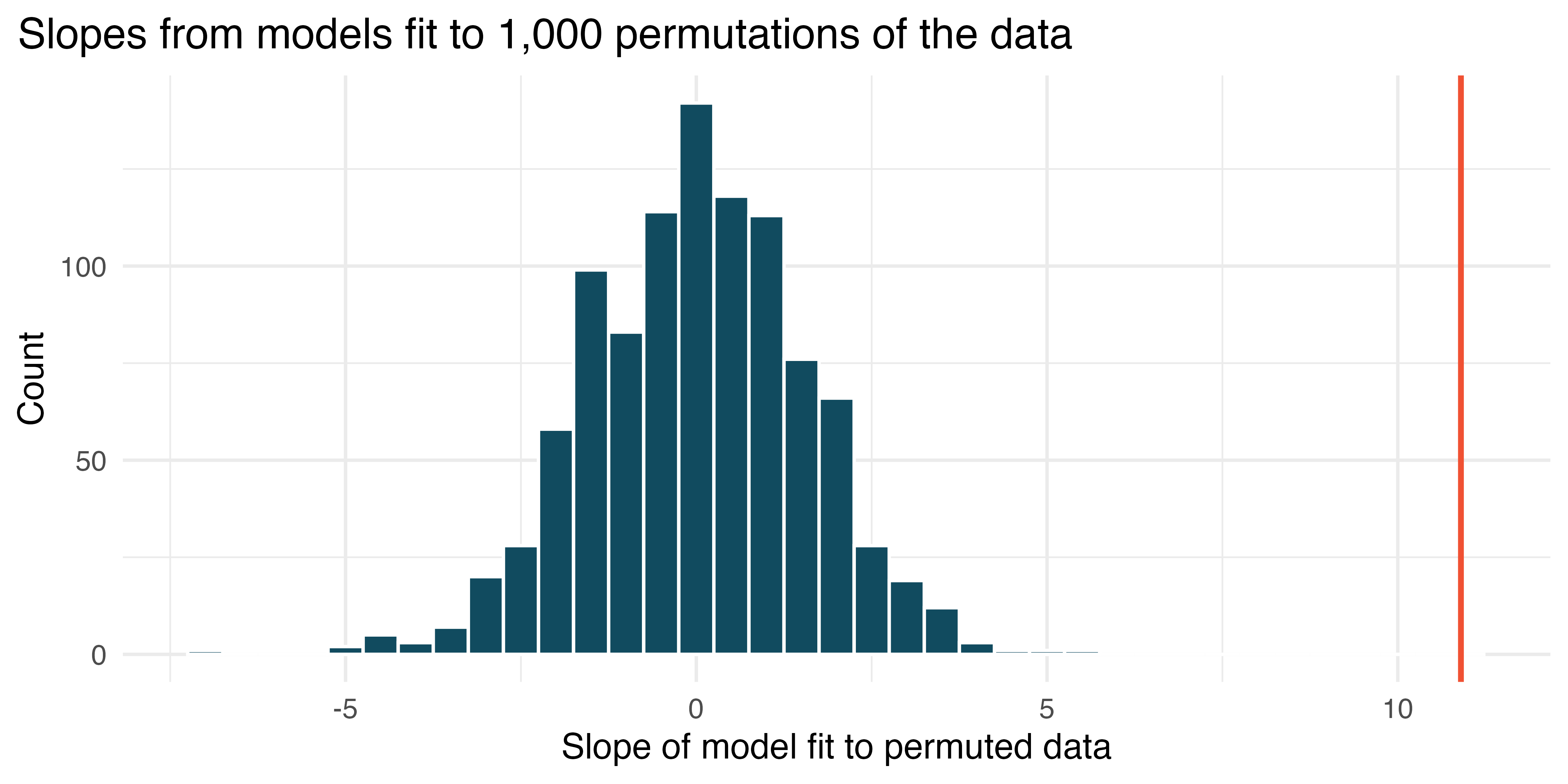
price regressed on cond_new) built on 1,000 randomized datasets. Each dataset was permuted under the null hypothesis.
In Figure 27.1, the red line (the observed slope) is far from the bulk of the histogram. Explain why the randomly permuted datasets produce slopes that are quite different from the observed slope.
The null hypothesis is that, in the population, there is no linear relationship between the price and the cond_new of the Mario Kart games. When the data are randomly permuted, prices are randomly assigned to a condition (new or used), so that the null hypothesis is forced to be true, i.e., permutation is done under the assumption that no relationship between the two variables exists. In the actual study, the new Mario Kart games do actually cost more (on average) than the used games! So the slope describing the actual observed relationship is not one that is likely to have happened in a randomly dataset permuted under the assumption that the null hypothesis is true.
Using the histogram in Figure 27.1, find the p-value and conclude the hypothesis test in the context of the problem.5
Is the conclusion based on the histogram of randomized slopes consistent with the conclusion obtained using the mathematical model? Explain.6
Although knowing there is a relationship between the condition of the game and its price, we might be more interested in the difference in price, here given by the slope of the linear regression line. That is, \(\beta_1\) represents the population value for the difference in price between new Mario Kart games and used games.
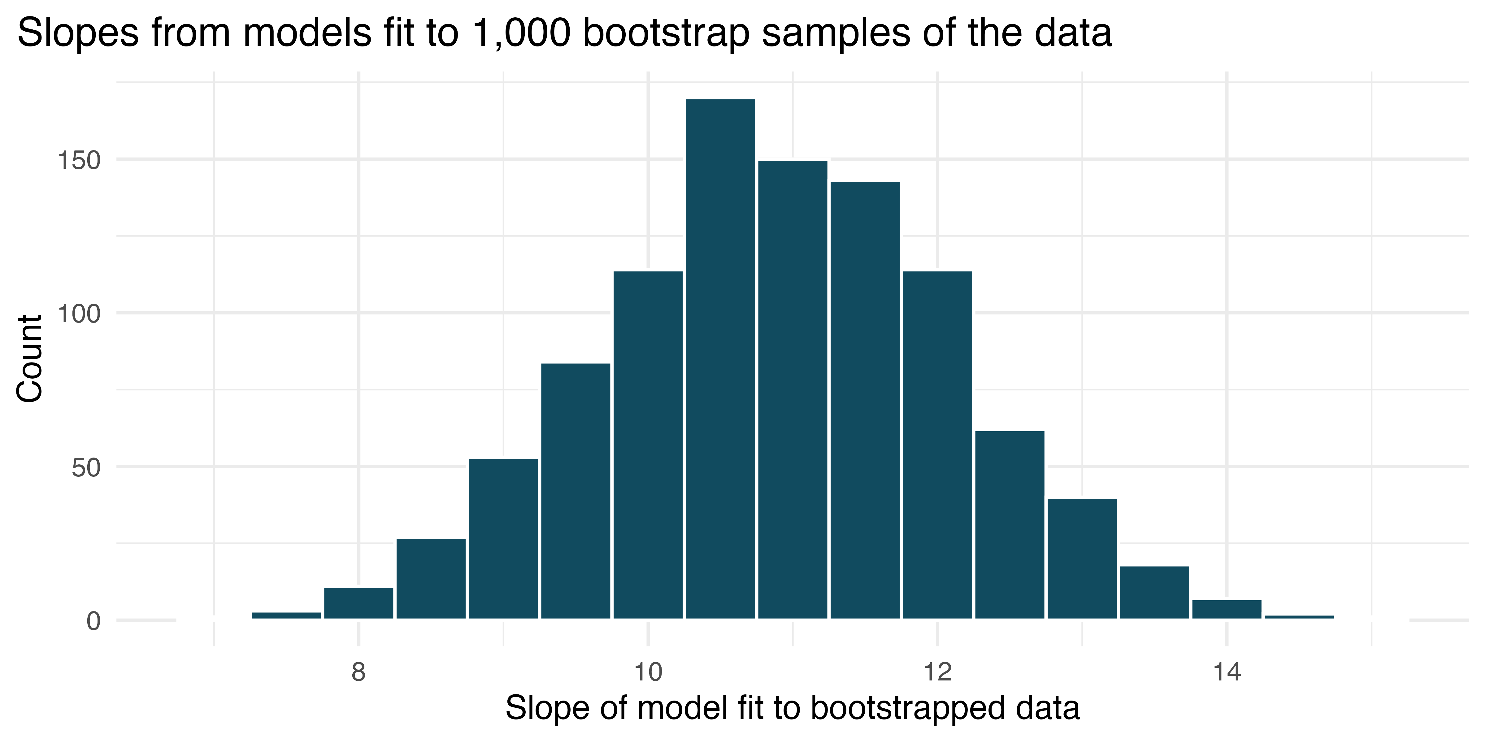
price regressed on cond_new) built on 1,000 bootstrapped datasets. Each bootstrap sample was taken from the original Mario Kart auction data.
Figure 27.2 displays the slope estimates taken from bootstrap samples of the original data. Using the histogram, estimate the standard error of the slope. Is your estimate similar to the value of the standard error of the slope provided in the output of the mathematical linear model?
The slopes seem to vary from approximately 8 to 14. Using the empirical rule, we know that if a variable has a bell-shaped distribution, most of the observations will be with 2 standard errors of the center. Therefore, a rough approximation of the standard error is 1.5. The standard error given in Table 27.3 is 1.26 which is not too different from the value computed using the bootstrap approach.
Use Figure 27.2 to create a 90% standard error bootstrap confidence interval for the true slope. Interpret the interval in context.7
Use Figure 27.2 to create a 90% bootstrap percentile confidence interval for the true slope. Interpret the interval in context.8
27.1.3 Cross-validation
In Chapter 8, models were compared using \(R^2_{adj}.\) In Chapter 25, however, a computational approach was introduced to compare models by removing chunks of data one at a time and assessing how well the variables predicted the observations that had been held out.
Figure 27.3 was created by cross-validating models with the same variables as in Table 27.3 and Table 27.4. We applied 3-fold cross-validation, so 1/3 of the data was removed while 2/3 of the observations were used to build each model (first on cond_new only and then on cond_new, stock_photo, duration, and wheels). Note that each time 1/3 of the data is removed, the resulting model will produce slightly different model coefficients.
The points in Figure 27.3 represent the prediction (x-axis) and residual (y-axis) for each observation run through the cross-validated model. In other words, the model is built (using the other 2/3) without the observation (which is in the 1/3) being used. The residuals give us a sense for how well the model will do at predicting observations which were not a part of the original dataset, e.g., future studies.
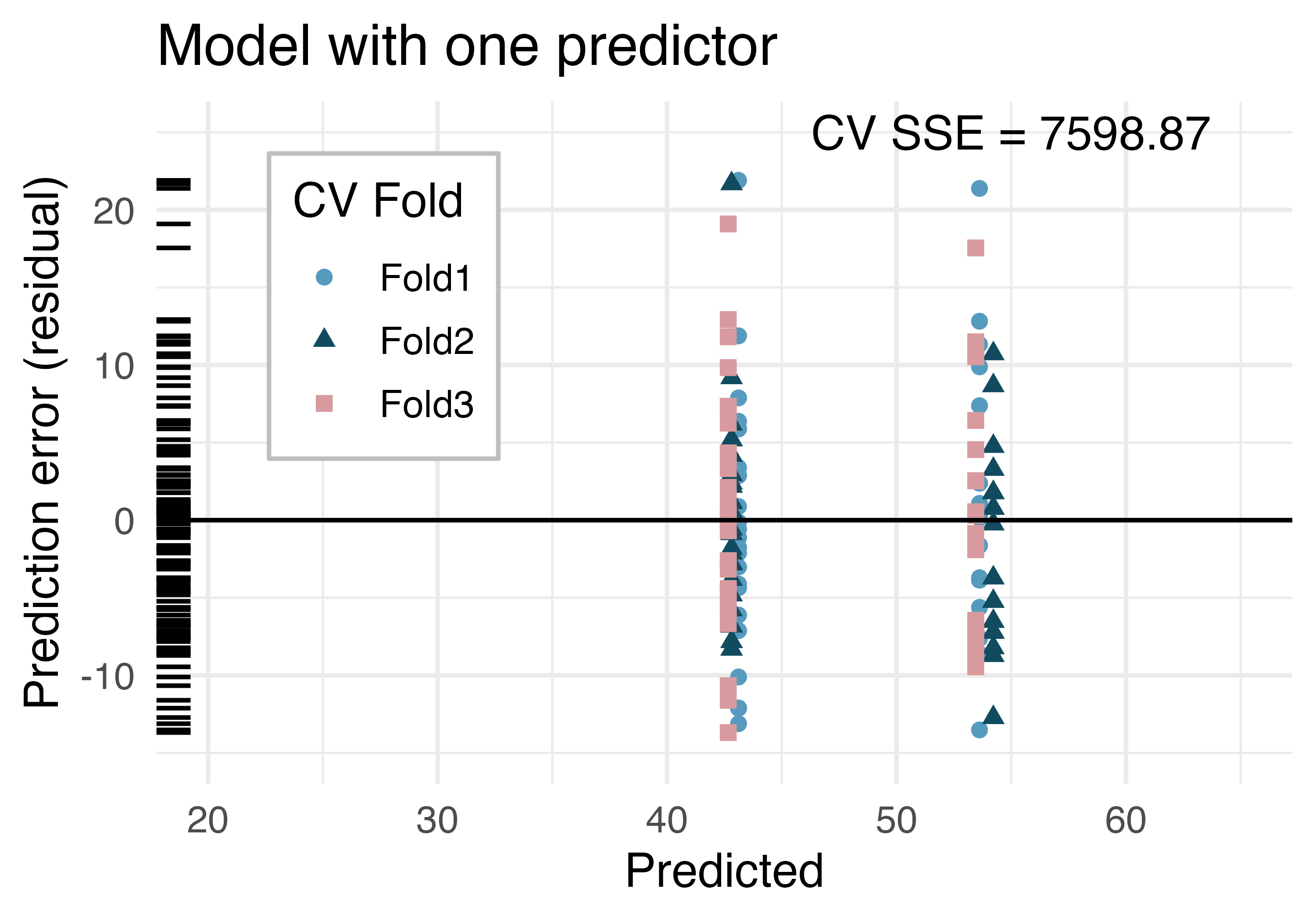
price vs. cond_new
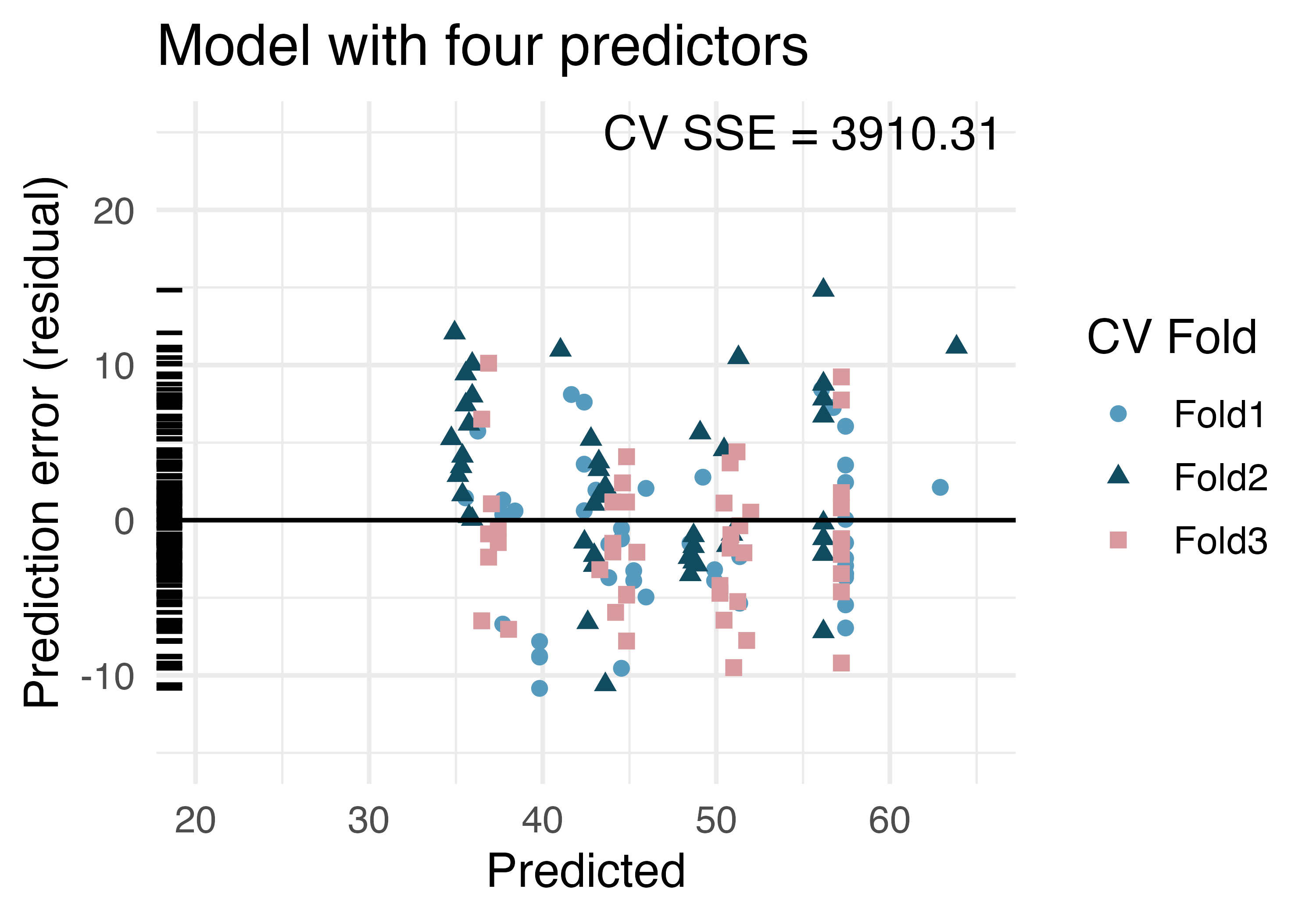
price vs. cond_new, stock_photo, duration, and wheels
In Figure 27.3 (b), note the point at roughly predicted = 50 and prediction error = 10. Estimate the observed and predicted value for that observation.9
In Figure 27.3 (b), for the same point at roughly predicted = 50 and prediction error = 10, describe which cross-validation fold(s) were used to build its prediction model.10
By noting the spread of the cross-validated prediction errors (on the y-axis) in Figure 27.3, which model should be chosen for a final report on these data?11
Using the summary statistic cross-validation sum of squared errors (CV SSE), which model should be chosen for a final report on these data?12
27.2 Interactive R tutorials
Navigate the concepts you’ve learned in this part in R using the following self-paced tutorials. All you need is your browser to get started!
You can also access the full list of tutorials supporting this book here.
27.3 R labs
Further apply the concepts you’ve learned in this part in R with computational labs that walk you through a data analysis case study.
You can also access the full list of labs supporting this book here.
The equation for the line may be written as \(\widehat{\texttt{price}} = 47.15 + 10.90\times \texttt{cond\_new}\). Examining the regression output in Table 27.3 we can see that the p-value for
cond_newis very close to zero, indicating there is strong evidence that the coefficient is different from zero when using this one-variable model. The variablecond_newis a two-level categorical variable that takes value 1 when the game is new and value 0 when the game is used. This means the 10.90 model coefficient predicts a price of an extra $10.90 for those games that are new versus those that are used.↩︎\(\widehat{\texttt{price}} = 36.21 + 5.13 \times \texttt{cond\_new} + 1.08 \times \texttt{stock\_photo} - 0.03 \times \texttt{duration} + 7.29 \times \texttt{wheels},\) with 4 predictors but 5 coefficients (including the intercept).↩︎
In the population of all auctions, it is the average difference in auction price for each additional Wii wheel included when holding the other variables constant. The point estimate is \(b_4 = 7.29\)↩︎
\(e_i = y_i - \hat{y_i} = 51.55 - 49.62 = 1.93\).↩︎
The observed slope is 10.9 which is nowhere near the range of values for the permuted slopes (roughly -5 to +5). Because the observed slope is not a plausible value under the null distribution, the p-value is essentially zero. We reject the null hypothesis and claim that there is a relationship between whether the game is new (or not) and the average predicted price of the game.↩︎
The p-value in Table 27.3 is also essentially zero, so the null hypothesis is also rejected when the mathematical model approach is taken. Often, the mathematical and computational approaches to inference will give quite similar answers.↩︎
Using the bootstrap SE method, we know the normal percentile is \(z^\star = 1.645\), which gives a CI of \(b_1 \pm 1.645 \cdot SE \rightarrow 10.9 \pm 1.645 \cdot 1.5 \rightarrow (8.43, 13.37).\) For games that are new, the average price is higher by between $8.43 and $13.37 than games that are used, with 90% confidence.↩︎
Because there were 1,000 bootstrap resamples, we look for the cutoffs which provide 50 bootstrap slopes on the left, 900 in the middle, and 50 on the right. Looking at the bootstrap histogram, the rough 90% confidence interval is $9 to $13.10. For games that are new, the average price is higher by between $9.00 and $13.10 than games that are used, with 90% confidence.↩︎
The predicted value is roughly \(\widehat{\texttt{price}} = \$50.\) The observed value is roughly \(\texttt{price}_i = \$60\) riders (using \(e_i = y_i - \hat{y}_i).\)↩︎
The point appears to be in fold 2, so folds 1 and 3 were used to build the prediction model.↩︎
The cross-validated residuals on
cond_newvary roughly from -15 to 15, while the cross-validated residuals on the four predictor model vary less, roughly from -10 to 10. Given the smaller residuals from the four predictor model, it seems as though the larger model is better.↩︎The CV SSE is smaller (by a factor of almost two!) for the model with four predictors. Using a single valued criterion (CV SSE) allows us to make a decision to choose the model with four predictors.↩︎