26 Inference for logistic regression
Combining ideas from Chapter 9 on logistic regression, Chapter 13 on inference with mathematical models, and Chapter 24 and Chapter 25 which apply inferential techniques to the linear model, we wrap up the book by considering inferential methods applied to a logistic regression model. Additionally, we use cross-validation as a method for independent assessment of the logistic regression model.
As with multiple linear regression, the inference aspect for logistic regression will focus on interpretation of coefficients and relationships between explanatory variables. Both p-values and cross-validation will be used for assessing a logistic regression model.
Consider the email data which describes email characteristics which can be used to predict whether a particular incoming email is spam (unsolicited bulk email). Without reading every incoming message, it might be nice to have an automated way to identify spam emails. Which of the variables describing each email are important for predicting the status of the email?
email dataset. Many of the variables are indicator variables, meaning they take the value 1 if the specified characteristic is present and 0 otherwise.
| Variable | Description |
|---|---|
| spam | Indicator for whether the email was spam. |
| to_multiple | Indicator for whether the email was addressed to more than one recipient. |
| from | Whether the message was listed as from anyone (this is usually set by default for regular outgoing email). |
| cc | Number of people cc'ed. |
| sent_email | Indicator for whether the sender had been sent an email in the last 30 days. |
| attach | The number of attached files. |
| dollar | The number of times a dollar sign or the word “dollar” appeared in the email. |
| winner | Indicates whether “winner” appeared in the email. |
| format | Indicates whether the email was written using HTML (e.g., may have included bolding or active links). |
| re_subj | Whether the subject started with “Re:”, “RE:”, “re:”, or “rE:” |
| exclaim_subj | Whether there was an exclamation point in the subject. |
| urgent_subj | Whether the word “urgent” was in the email subject. |
| exclaim_mess | The number of exclamation points in the email message. |
| number | Factor variable saying whether there was no number, a small number (under 1 million), or a big number. |
26.1 Model diagnostics
Before looking at the hypothesis tests associated with the coefficients (turns out they are very similar to those in linear regression!), it is valuable to understand the technical conditions that underlie the inference applied to the logistic regression model. Generally, as you’ve seen in the logistic regression modeling examples, it is imperative that the response variable is binary. Additionally, the key technical condition for logistic regression has to do with the relationship between the predictor variables (\(x_i\) values) and the probability the outcome will be a success. It turns out, the relationship is a specific functional form called a logit function, where \({\rm logit}(p) = \log_e(\frac{p}{1-p}).\) The function may feel complicated, and memorizing the formula of the logit is not necessary for understanding logistic regression. What you do need to remember is that the probability of the outcome being a success is a function of a linear combination of the explanatory variables.
Logistic regression conditions.
There are two key conditions for fitting a logistic regression model:
- Each outcome \(Y_i\) is independent of the other outcomes.
- Each predictor \(x_i\) is linearly related to logit\((p_i)\) if all other predictors are held constant.
The first logistic regression model condition — independence of the outcomes — is reasonable if we can assume that the emails that arrive in an inbox within a few months are independent of each other with respect to whether they’re spam or not.
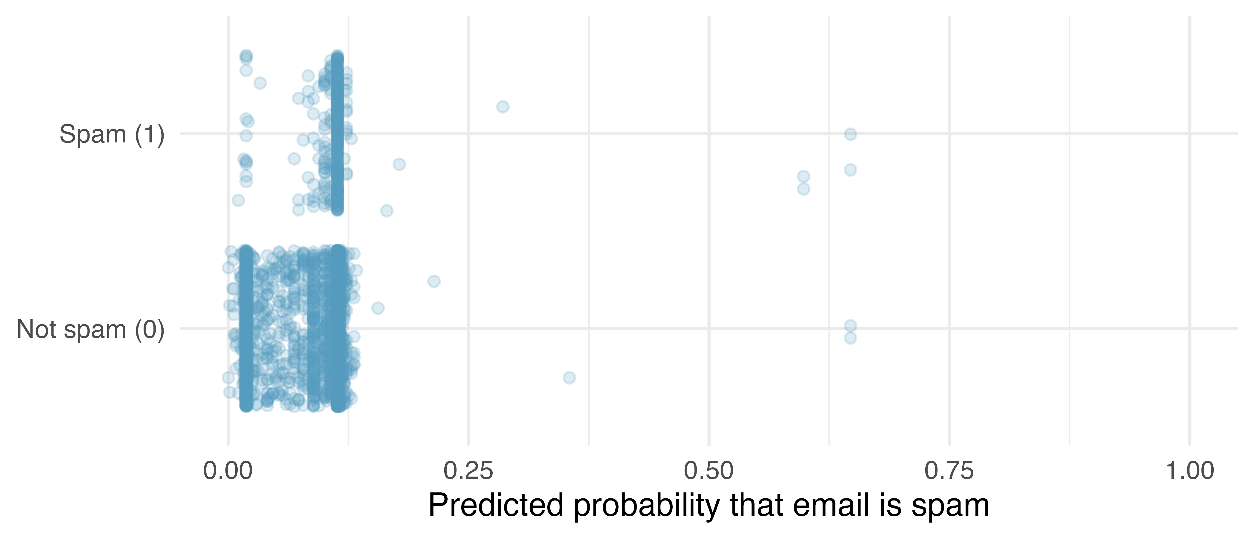
The second condition of the logistic regression model is not easily checked without a fairly sizable amount of data. Luckily, we have 3921 emails in the dataset! Let’s first visualize these data by plotting the true classification of the emails against the model’s fitted probabilities, as shown in Figure 26.1.
We’d like to assess the quality of the model. For example, we might ask: if we look at emails that we modeled as having 10% chance of being spam, do we find out 10% of them actually are spam? We can check this for groups of the data by constructing a plot as follows:
- Bucket the observations into groups based on their predicted probabilities.
- Compute the average predicted probability for each group.
- Compute the observed probability for each group, along with a 95% confidence interval for the true probability of success for those individuals.
- Plot the observed probabilities (with 95% confidence intervals) against the average predicted probabilities for each group.
If the model does a good job describing the data, the plotted points should fall close to the line \(y = x\), since the predicted probabilities should be similar to the observed probabilities. We can use the confidence intervals to roughly gauge whether anything might be amiss. Such a plot is shown in Figure 26.2.
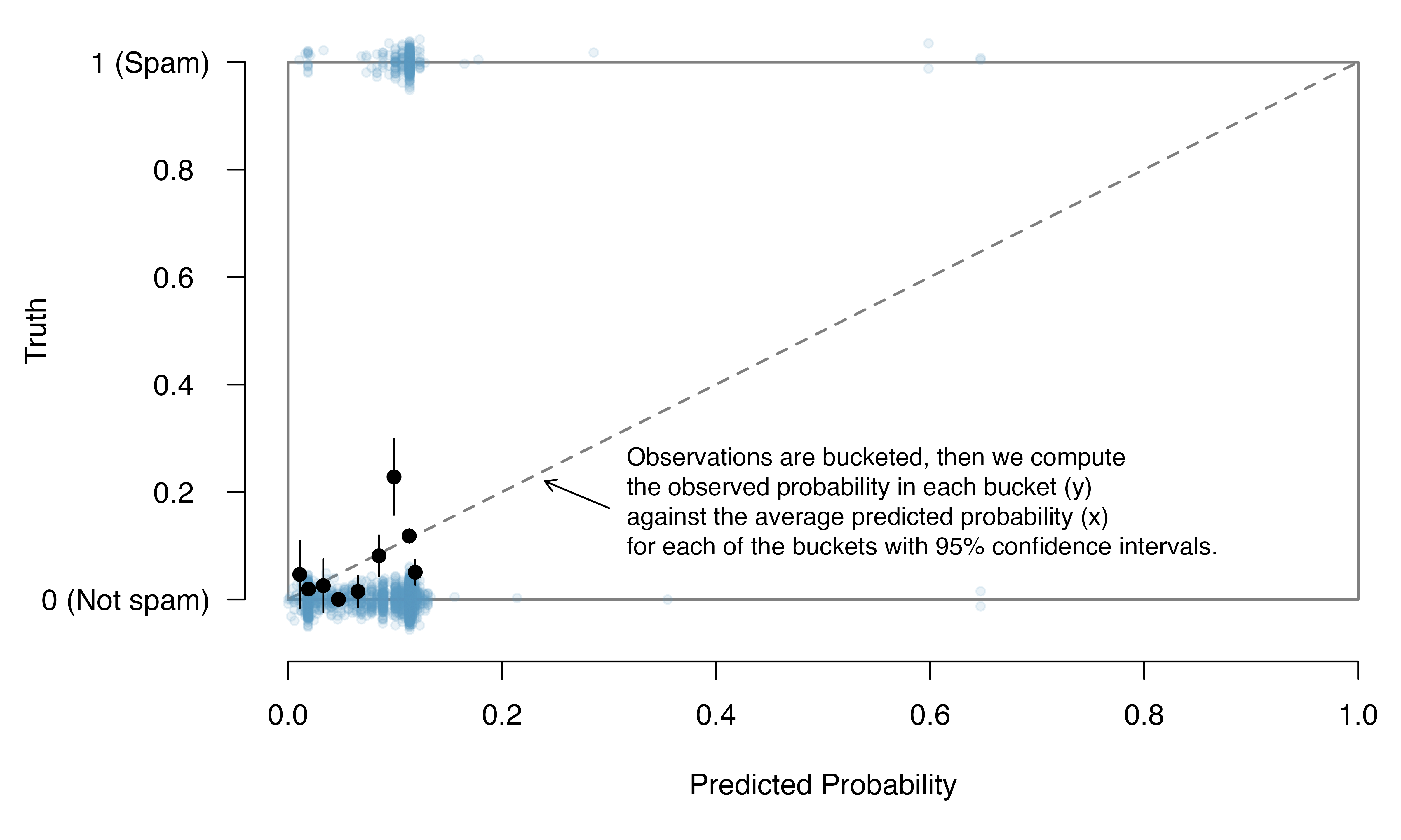
A plot like Figure 26.2 helps to better understand the deviations. Additional diagnostics may be created that are similar to those featured in Section 24.6. For instance, we could compute residuals as the observed outcome minus the expected outcome (\(e_i = Y_i - \hat{p}_i\)), and then we could create plots of these residuals against each predictor.
26.2 Multiple logistic regression output from software
As you learned in Chapter 8, optimization can be used to find the coefficient estimates for the logistic model. The unknown population model can be written as:
\[ \begin{aligned} \log_e\bigg(\frac{p}{1-p}\bigg) = \beta_0 &+ \beta_1 \times \texttt{to\_multiple}\\ &+ \beta_2 \times \texttt{cc} \\ &+ \beta_3 \times \texttt{dollar}\\ &+ \beta_4 \times \texttt{urgent\_subj} \end{aligned} \]
The estimated equation for the regression model may be written as a model with four predictor variables, where \(\hat{p}\) is the estimated probability of being a spam email message:
\[ \begin{aligned} \log_e\bigg(\frac{\hat{p}}{1-\hat{p}}\bigg) = -2.05 &-1.91 \times \texttt{to\_multiple}\\ &+ 0.02 \times \texttt{cc} \\ &- 0.07 \times \texttt{dollar}\\ &+ 2.66 \times \texttt{urgent\_subj} \end{aligned} \]
| term | estimate | std.error | statistic | p.value |
|---|---|---|---|---|
| (Intercept) | -2.05 | 0.06 | -34.67 | <0.0001 |
| to_multiple1 | -1.91 | 0.30 | -6.37 | <0.0001 |
| cc | 0.02 | 0.02 | 1.16 | 0.245 |
| dollar | -0.07 | 0.02 | -3.38 | 7e-04 |
| urgent_subj1 | 2.66 | 0.80 | 3.32 | 9e-04 |
Not only does Table 26.2 provide the estimates for the coefficients, it also provides information on the inference analysis (i.e., hypothesis testing) which is the focus of this chapter.
As in Chapter 25, with multiple predictors, each hypothesis test (for each of the explanatory variables) is conditioned on each of the other variables remaining in the model.
if multiple predictors \(H_0: \beta_i = 0\) given other variables in the model
Using the example above and focusing on each of the variable p-values (here we won’t discuss the p-value associated with the intercept), we can write out the four different hypotheses (associated with the p-value corresponding to each of the coefficients / rows in Table 26.2):
-
\(H_0: \beta_1 = 0\) given
cc,dollar, andurgent_subjare included in the model -
\(H_0: \beta_2 = 0\) given
to_multiple,dollar, andurgent_subjare included in the model -
\(H_0: \beta_3 = 0\) given
to_multiple,cc, andurgent_subjare included in the model -
\(H_0: \beta_4 = 0\) given
to_multiple,cc, anddollarare included in the model
The very low p-values from the software output tell us that three of the variables (that is, not cc) act as statistically discernible predictors in the model at the discernibility level of 0.05, despite the inclusion of any of the other variables. Consider the p-value on \(H_0: \beta_1 = 0\). The low p-value says that it would be extremely unlikely to observe data that yield a coefficient on to_multiple at least as far from 0 as -1.91 (i.e., \(|b_1| > 1.91\)) if the true relationship between to_multiple and spam was non-existent (i.e., if \(\beta_1 = 0\)) and the model also included cc and dollar and urgent_subj. Note also that the coefficient on dollar has a small associated p-value, but the magnitude of the coefficient is also seemingly small (0.07). It turns out that in units of standard errors (0.02 here), 0.07 is actually quite far from zero, it’s all about context! The p-values on the remaining variables are interpreted similarly. From the initial output (p-values) in Table 26.2, it seems as though to_multiple, dollar, and urgent_subj are important variables for modeling whether an email is spam. We remind you that although p-values provide some information about the importance of each of the predictors in the model, there are many, arguably more important, aspects to consider when choosing the best model.
As with linear regression (see Section 25.2), existence of predictors that are correlated with each other can affect both the coefficient estimates and the associated p-values. However, investigating multicollinearity in a logistic regression model is saved for a text which provides more detail about logistic regression. Next, as a model building alternative (or enhancement) to p-values, we revisit cross-validation within the context of predicting status for each of the individual emails.
26.3 Cross-validation for prediction error
The p-value is a probability measure under a setting of no relationship. That p-value provides information about the degree of the relationship (e.g., above we measure the relationship between spam and to_multiple using a p-value), but the p-value does not measure how well the model will predict the individual emails (e.g., the accuracy of the model). Depending on the goal of the research project, you might be inclined to focus on variable importance (through p-values) or you might be inclined to focus on prediction accuracy (through cross-validation).
Here we present a method for using cross-validation accuracy to determine which variables (if any) should be used in a model which predicts whether an email is spam. A full treatment of cross-validation and logistic regression models is beyond the scope of this text. Using \(k\)-fold cross-validation, we can build \(k\) different models which are used to predict the observations in each of the \(k\) holdout samples. As with linear regression (see Section 25.3), we compare a smaller logistic regression model to a larger logistic regression model. The smaller model uses only the to_multiple variable, see the complete dataset (not cross-validated) model output in Table 26.3. The logistic regression model can be written as follows, where \(\hat{p}\) is the estimated probability of being a spam email message.
The smaller model:
\[\log_e\bigg(\frac{\hat{p}}{1-\hat{p}}\bigg) = -2.12 + -1.81 \times \texttt{to\_multiple}\]
| term | estimate | std.error | statistic | p.value |
|---|---|---|---|---|
| (Intercept) | -2.12 | 0.06 | -37.67 | <0.0001 |
| to_multiple1 | -1.81 | 0.30 | -6.09 | <0.0001 |
For each cross-validated model, the coefficients change slightly, and the model is used to make independent predictions on the holdout sample. The model from the first cross-validation sample is given in Figure 26.3 and can be compared to the coefficients in Table 26.3.
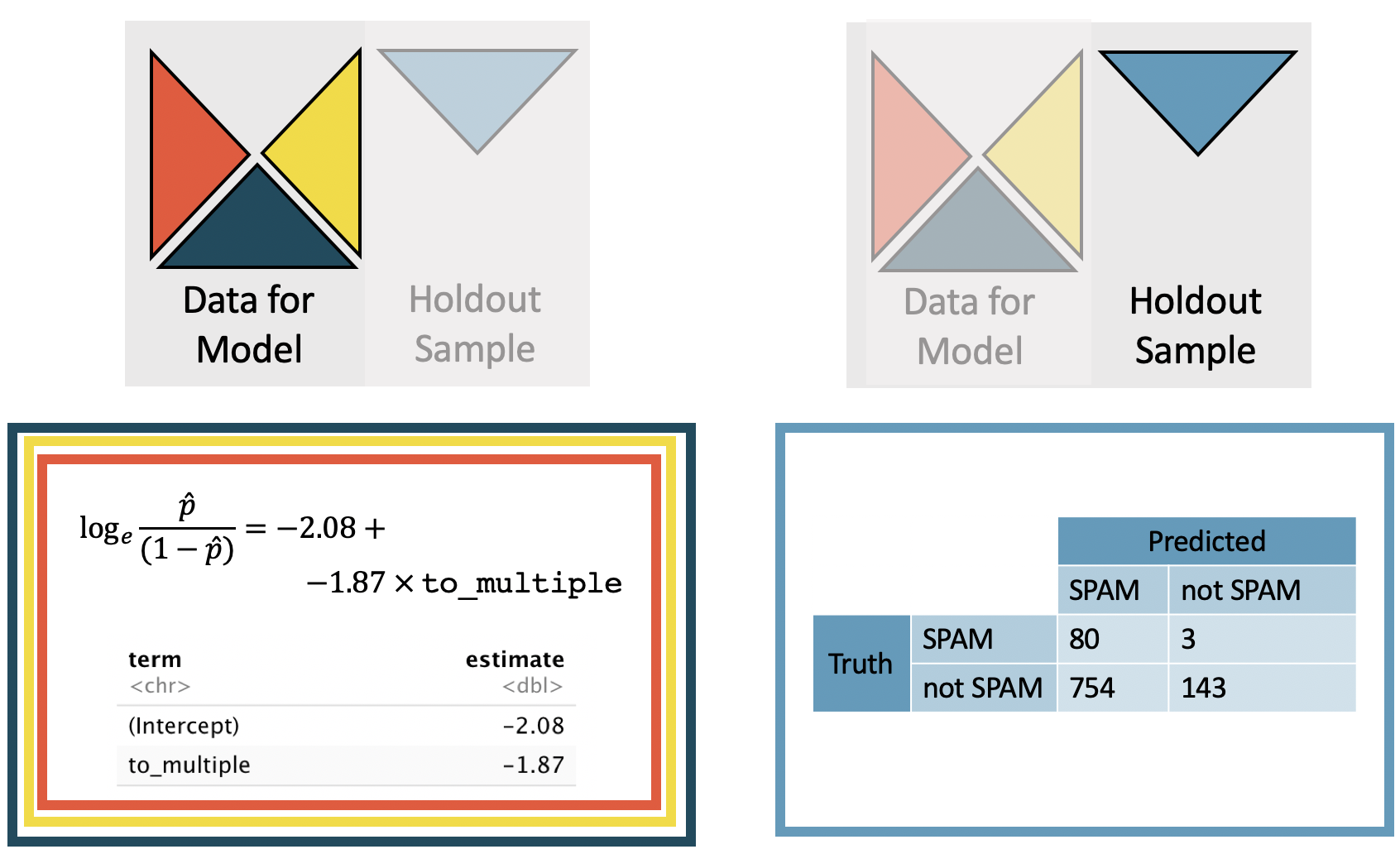
to_multiple is used to predict whether the email is spam. Because we used a cutoff designed to identify spam emails, the accuracy of the non-spam email predictions is very low. spamTP is the proportion of true spam emails that were predicted to be spam. notspamTP is the proportion of true not spam emails that were predicted to be not spam.
| fold | count | accuracy | notspamTP | spamTP |
|---|---|---|---|---|
| 1st quarter | 980 | 0.26 | 0.19 | 0.98 |
| 2nd quarter | 981 | 0.23 | 0.15 | 0.96 |
| 3rd quarter | 979 | 0.25 | 0.18 | 0.96 |
| 4th quarter | 981 | 0.24 | 0.17 | 0.98 |
Because the email dataset has a ratio of roughly 90% non-spam and 10% spam emails, a model which randomly guessed all non-spam would have an overall accuracy of 90%! Clearly, we would like to capture the information with the spam emails, so our interest is in the percent of spam emails which are identified as spam (see Table 26.4). Additionally, in the logistic regression model, we use a 10% cutoff to predict whether the email is spam. Fortunately, we have done a great job of predicting! However, the trade-off was that most of the non-spam emails are now predicted to be spam which is not acceptable for a prediction algorithm. Adding more variables to the model may help with both the spam and non-spam predictions.
The larger model uses to_multiple, attach, winner, format, re_subj, exclaim_mess, and number as the set of seven predictor variables, see the complete dataset (not cross-validated) model output in Table 26.5. The logistic regression model can be written as follows, where \(\hat{p}\) is the estimated probability of being a spam email message.
The larger model:
\[ \begin{aligned} \log_e\bigg(\frac{\hat{p}}{1-\hat{p}}\bigg) = -0.34 &- 2.56 \times \texttt{to\_multiple} + 0.20 \times \texttt{attach} + 1.73 \times \texttt{winner}_{yes} \\ &- 1.28 \times \texttt{format} - 2.86 \times \texttt{re\_subj} + 0.00 \times \texttt{exclaim\_mess} \\ &- 1.07 \times \texttt{number}_{small} - 0.42 \times \texttt{number}_{big} \end{aligned} \]
to_multiple, attach, winner, format, re_subj, exclaim_mess, and number. Each of the variables has its own coefficient estimate and p-value.
| term | estimate | std.error | statistic | p.value |
|---|---|---|---|---|
| (Intercept) | -0.34 | 0.11 | -3.02 | 0.0025 |
| to_multiple1 | -2.56 | 0.31 | -8.28 | <0.0001 |
| attach | 0.20 | 0.06 | 3.29 | 0.001 |
| winneryes | 1.73 | 0.33 | 5.33 | <0.0001 |
| format1 | -1.28 | 0.13 | -9.80 | <0.0001 |
| re_subj1 | -2.86 | 0.37 | -7.83 | <0.0001 |
| exclaim_mess | 0.00 | 0.00 | 0.26 | 0.7925 |
| numbersmall | -1.07 | 0.14 | -7.54 | <0.0001 |
| numberbig | -0.42 | 0.20 | -2.10 | 0.0357 |
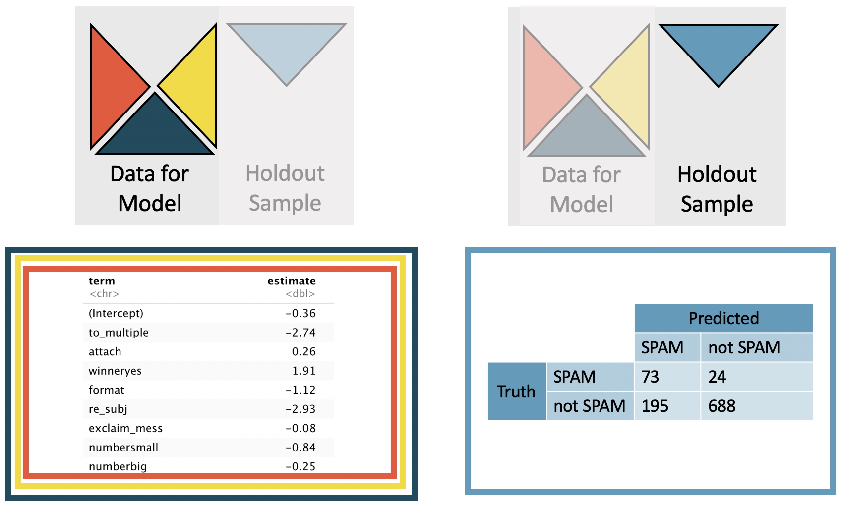
to_multiple, attach, winner, format, re_subj, exclaim_mess, and number are used to predict whether the email is spam. spamTP is the proportion of true spam emails that were predicted to be spam. notspamTP is the proportion of true not spam emails that were predicted to be not spam.’
| fold | count | accuracy | notspamTP | spamTP |
|---|---|---|---|---|
| 1st quarter | 980 | 0.77 | 0.77 | 0.71 |
| 2nd quarter | 981 | 0.80 | 0.81 | 0.70 |
| 3rd quarter | 979 | 0.76 | 0.77 | 0.65 |
| 4th quarter | 981 | 0.78 | 0.79 | 0.75 |
Somewhat expected, the larger model (see Table 26.6) was able to capture more nuance in the emails which lead to better predictions. However, it is not true that adding variables will always lead to better predictions, as correlated or noise variables may dampen the signal from the set of variables that truly predict the status. We encourage you to learn more about multiple variable models and cross-validation in your future exploration of statistical topics.
26.4 Chapter review
26.4.1 Summary
Throughout the text, we have presented a modern view to introduction to statistics. Earlier, we presented graphical techniques which communicated relationships across multiple variables. We also used modeling to formalize the relationships. In Chapter 26 we considered inferential claims on models which include many variables used to predict the probability of the outcome being a success. We continue to emphasize the importance of experimental design in making conclusions about research claims. In particular, recall that variability can come from different sources (e.g., random sampling vs. random allocation, see Figure 2.8).
As you might guess, this text has only scratched the surface of the world of statistical analyses that can be applied to different datasets. In particular, to do justice to the topic, the linear models and generalized linear models we have introduced can each be covered with their own course or book. Hierarchical models, alternative methods for fitting parameters (e.g., Ridge Regression or LASSO), and advanced computational methods applied to multivariable models (e.g., permuting the response variable? one explanatory variable? all the explanatory variables?) are all beyond the scope of this book. However, your successful understanding of the ideas we have covered has set you up perfectly to move on to a higher level of statistical modeling and inference. Enjoy!
26.4.2 Terms
The terms introduced in this chapter are presented in Table 26.7. If you’re not sure what some of these terms mean, we recommend you go back in the text and review their definitions. You should be able to easily spot them as bolded text.
| accuracy | inference on logistic regression | technical conditions |
| cross-validation | multiple predictors |
26.5 Exercises
Answers to odd-numbered exercises can be found in Appendix A.26.
- Passing the driver’s test. A consulting company is hired to assess whether certain characteristics of a DMV (e.g., location, number of test takers, number of test givers, hours of operation, etc.) are associated with the pass rate of the driver’s test. The company is given information on 100 randomly selected DMVs across the country. For each DMV the annual driving test pass rate is recorded, along with other characteristics describing the DMV. Can logistic regression with multiple predictors be used to predict annual driving test pass rate for DMVs in this setting? Explain your reasoning.
-
Oceans and skin cancer. A researcher wants to investigate the relationship between living within 10 miles of an ocean for at least one year of life and developing skin cancer before the age of 50.
Explain why logistic regression can be used to study the relationship between these two binary variables? What is the technical assumption describing the relationship between the response (outcome) and explanatory (predictor) variables?
What other methods covered in this text might be used to address the research question of interest? What advantages does logistic regression have over these methods?
-
Marijuana use in college. Researchers studying whether the value systems of adolescents conflict with those of their parents asked 445 college students if they use marijuana. They also asked the students’ parents if they used marijuana when they were in college. Based on the regression output shown below for predicting student drug use from parent drug use, evaluate whether parents’ marijuana usage is a discernible predictor of their kids’ marijuana usage. State the hypotheses, the test statistics, the p-value, and the conclusion in context of the data and the research question.1 (Ellis and Stone 1979)
term estimate std.error statistic p.value (Intercept) -0.405 0.133 -3.04 0.0023 parentsused 0.791 0.194 4.09 <0.0001
-
Treating heart attacks. Researchers studying the effectiveness of Sulfinpyrazone in the prevention of sudden death after a heart attack conducted a randomized experiment on 1,475 patients. Based on the regression output shown below for predicting the outcome (
diedorlived, where success is defined aslived) from the treatment group (controlandtreatment), evaluate whether treatment group is a discernible predictor of the outcome. State the hypotheses, the test statistics, the p-value, and the conclusion in context of the data and the research question.2 (Anturane Reinfarction Trial Research Group 1980)term estimate std.error statistic p.value (Intercept) 2.431 0.135 18.05 <0.0001 grouptreatment 0.395 0.210 1.89 0.0594
-
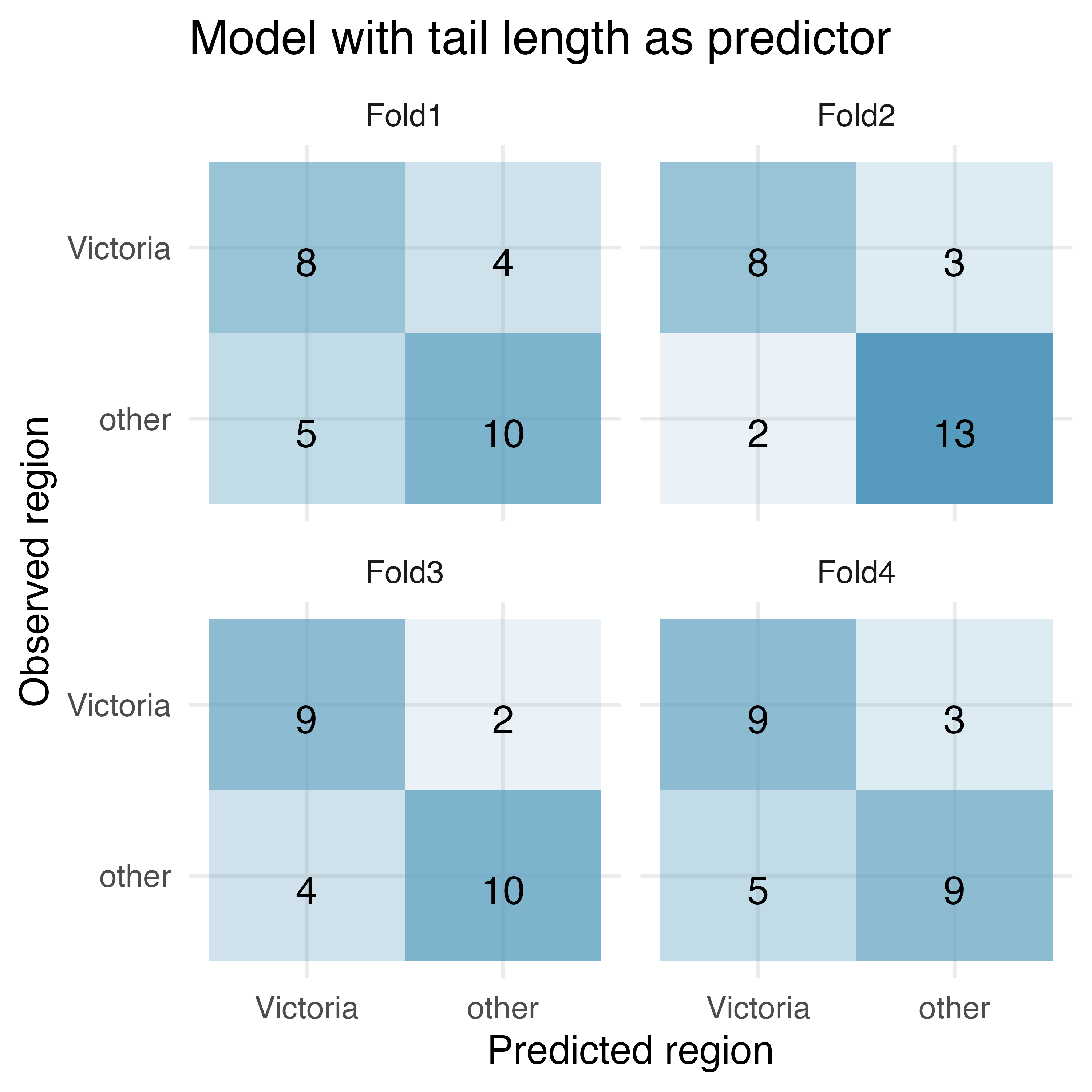
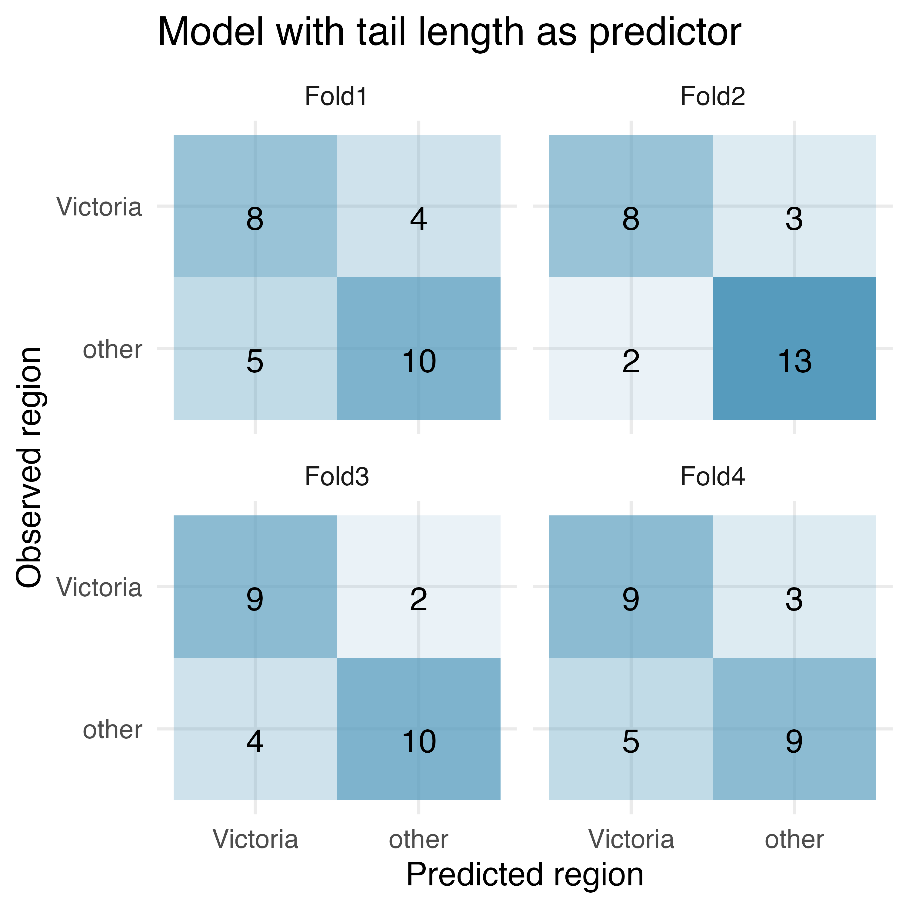
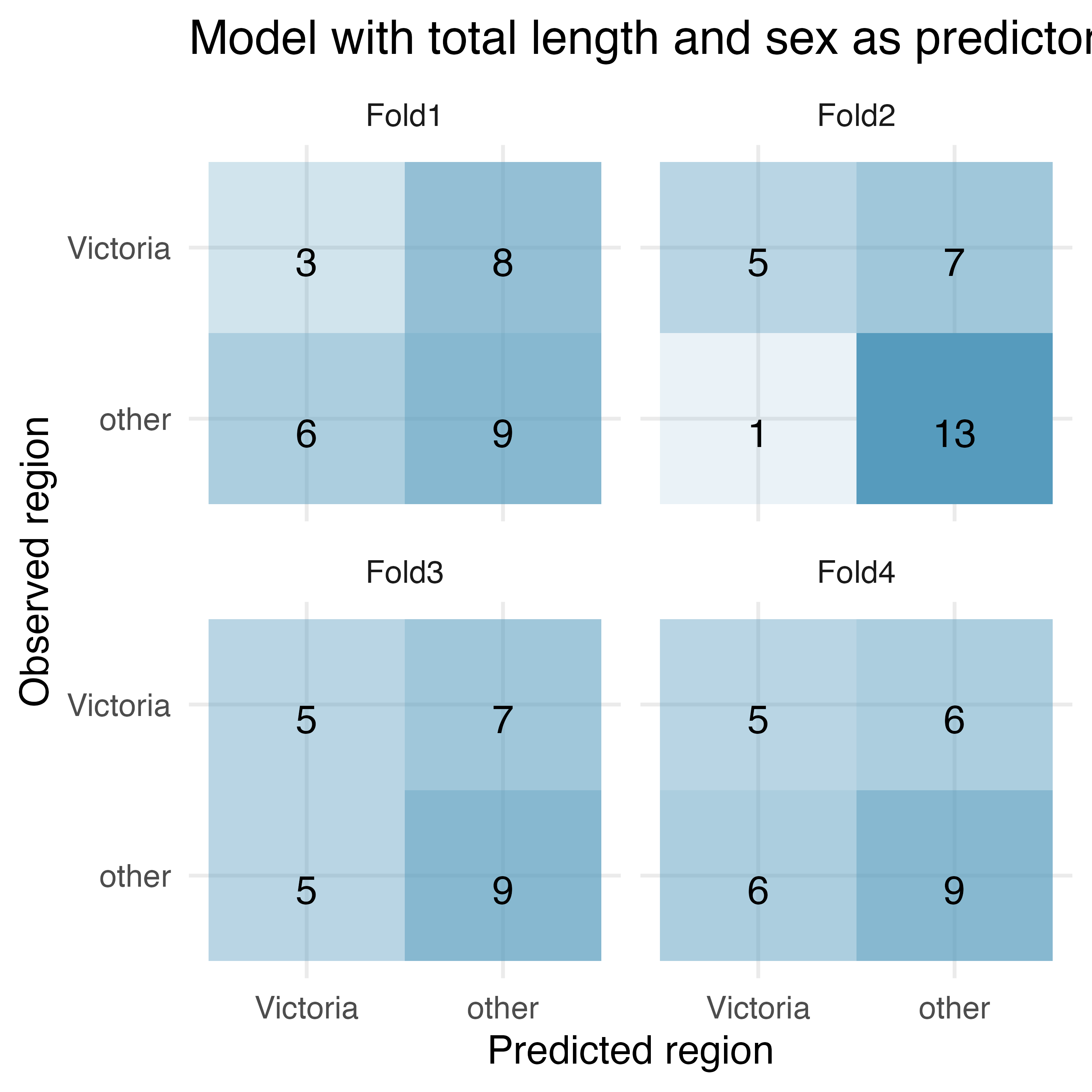
Possum classification, cross-validation. The common brushtail possum of the Australia region is a bit cuter than its distant cousin, the American opossum. We consider 104 brushtail possums from two regions in Australia, where the possums may be considered a random sample from the population. The first region is Victoria, which is in the eastern half of Australia and traverses the southern coast. The second region consists of New South Wales and Queensland, which make up eastern and northeastern Australia. We use logistic regression to differentiate between possums in these two regions. The outcome variable, called
pop, takes value 1 when a possum is from Victoria and 0 when it is from New South Wales or Queensland.3\[ \log_e \bigg(\frac{p}{1-p}\bigg) = \beta_0 + \beta_1 \times \texttt{tail\_l} \]
\[ \log_e \bigg(\frac{p}{1-p}\bigg) = \beta_0 + \beta_1 \times \texttt{total\_l} + \beta_2\times \texttt{sex} \]
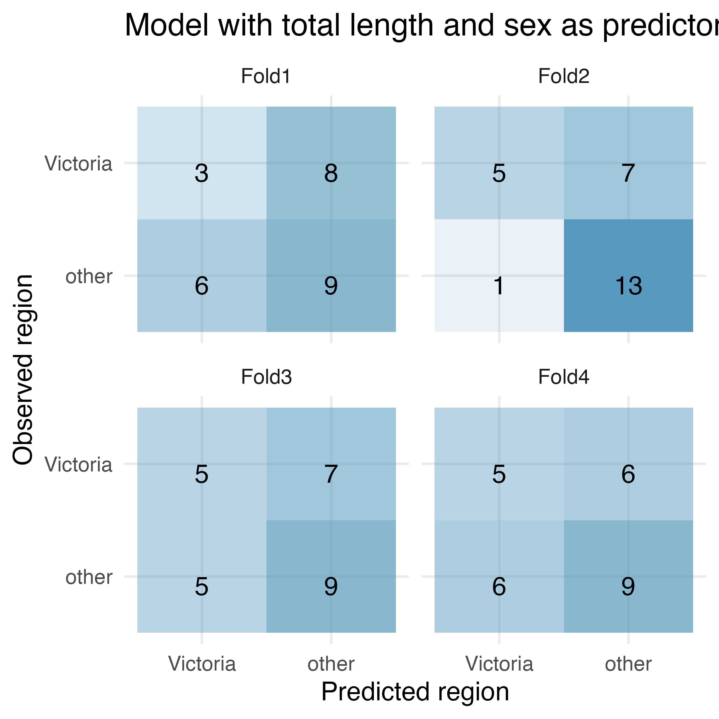
How many observations are in Fold2? Use the model with only tail length as a predictor variable. Of the observations in Fold2, how many of them were correctly predicted to be from Victoria? How many of them were incorrectly predicted to be from Victoria?
How many observations are used to build the model which predicts for the observations in Fold2?
For one of the cross-validation folds, how many coefficients were estimated for the model which uses tail length as a predictor? For one of the cross-validation folds, how many coefficients were estimated for the model which uses total length and sex as predictors?
-
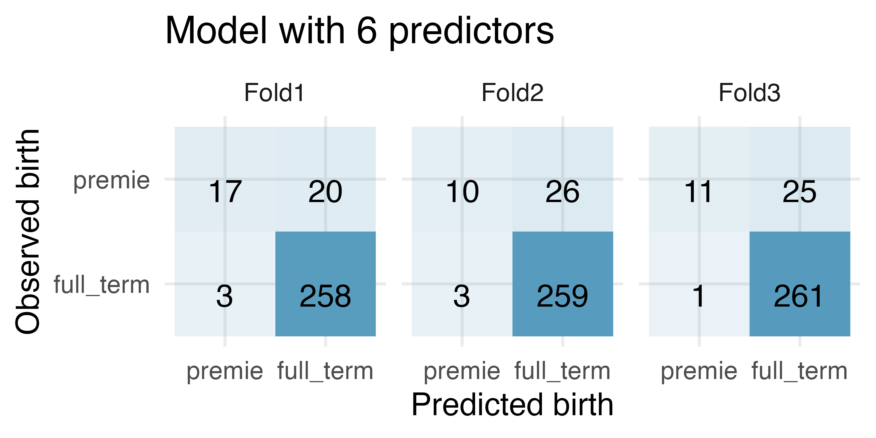
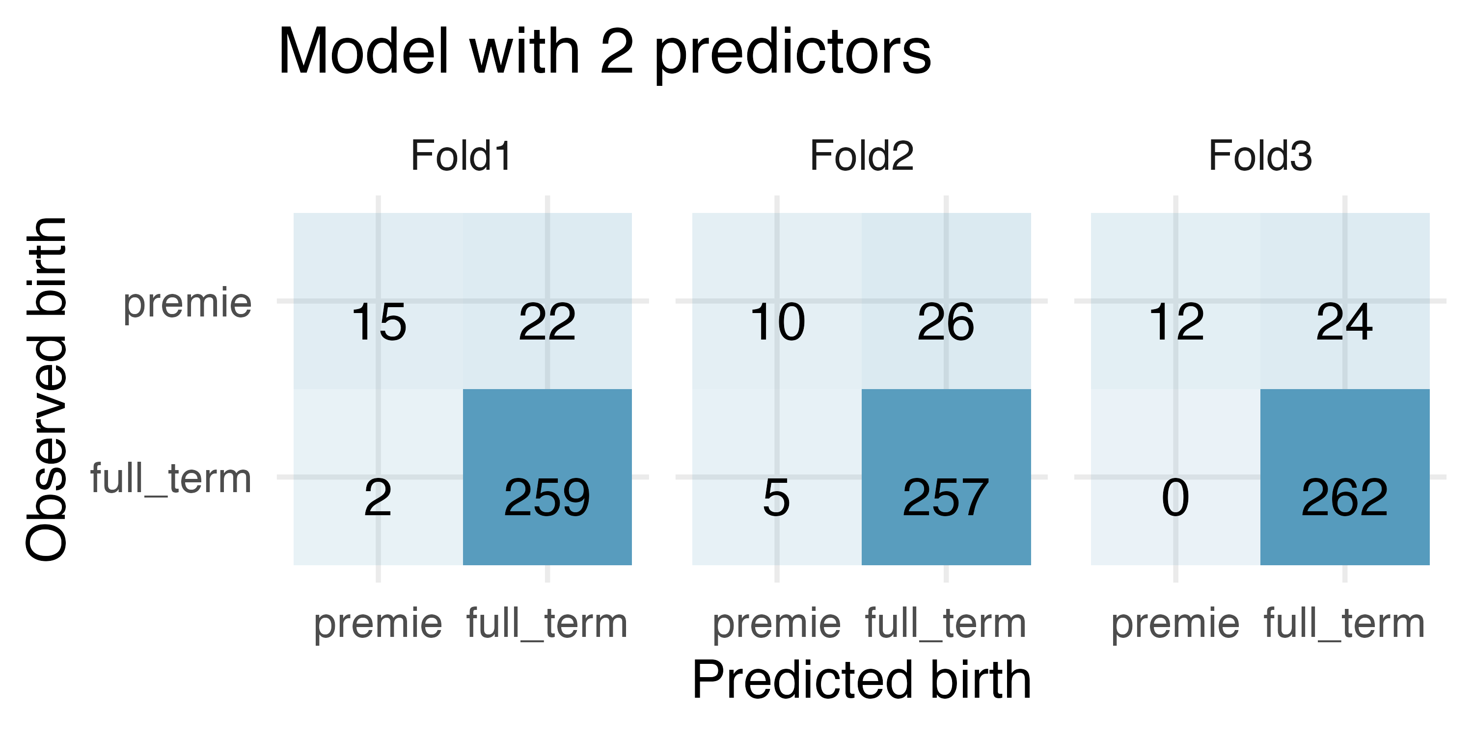
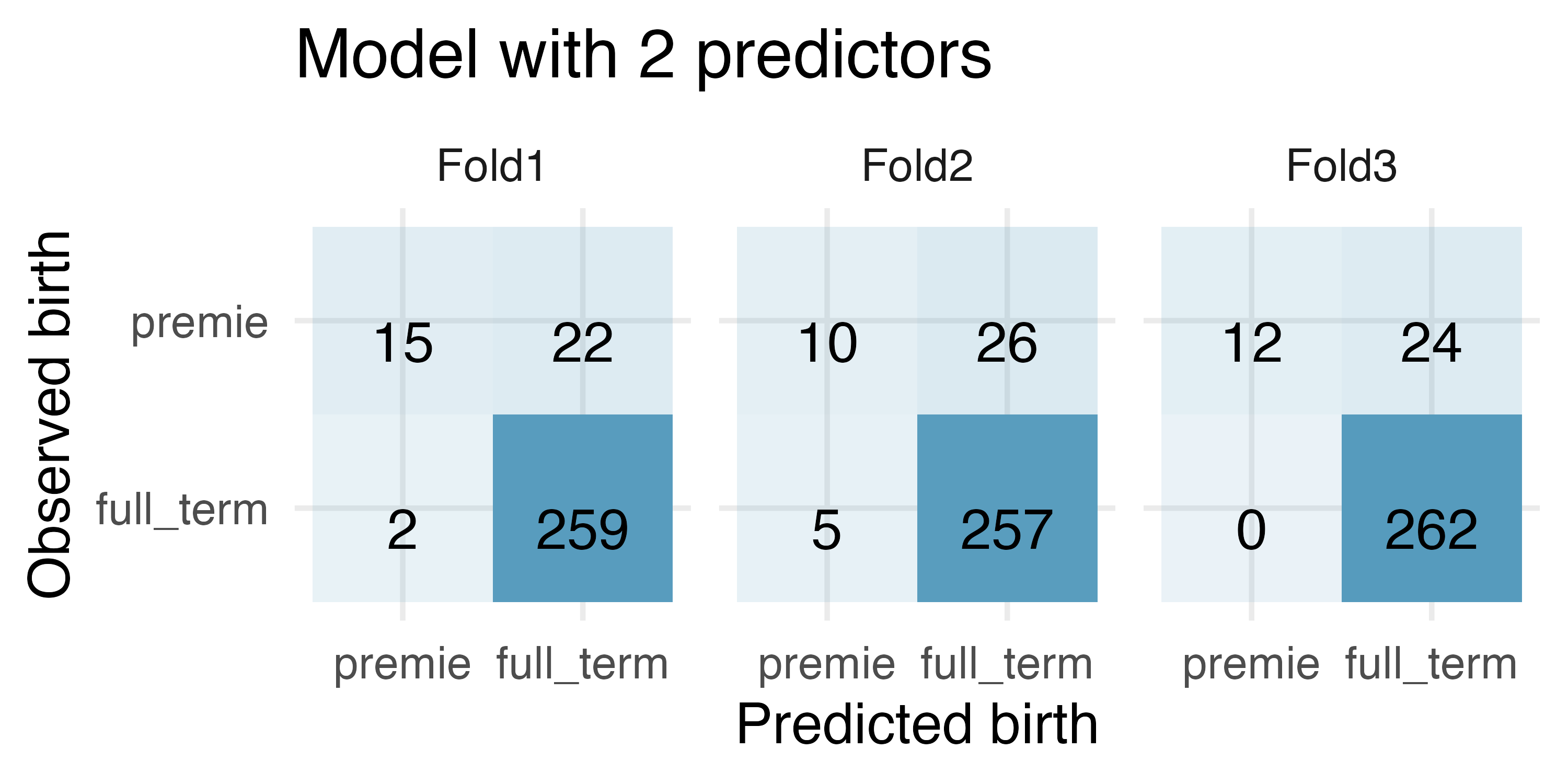
Premature babies, cross-validation. US Department of Health and Human Services, Centers for Disease Control and Prevention collect information on births recorded in the country. The data used here are a random sample of 1000 births from 2014 (with some rows removed due to missing data). We use logistic regression to model whether the baby is premature from various explanatory variables.4 (ICPSR 2014)
\[ \begin{aligned} \log_e \bigg(\frac{p}{1-p}\bigg) = \beta_0 &+ \beta_1\times \texttt{mage} \\ &+ \beta_2 \times \texttt{weight} \\ &+ \beta_3 \times \texttt{mature} \\ &+ \beta_4 \times \texttt{visits} \\ &+ \beta_5 \times \texttt{gained} \\ &+ \beta_6 \times \texttt{habit} \end{aligned} \]
\[ \begin{aligned} \log_e \bigg(\frac{p}{1-p}\bigg) = \beta_0 &+ \beta_1\times \texttt{weight} \\ &+ \beta_2 \times \texttt{mature} \end{aligned} \]
How many observations are in Fold2? Use the model with only
weightandmatureas predictor variables. Of the observations in Fold2, how many of them were correctly predicted to be premature? How many of them were incorrectly predicted to be premature?How many observations are used to build the model which predicts for the observations in Fold2?
In the original dataset, are most of the births premature or full term? Explain.
For one of the cross-validation folds, how many coefficients were estimated for the model which uses
mage,weight,mature,visits,gained, andhabitas predictors? For one of the cross-validation folds, how many coefficients were estimated for the model which usesweightandmatureas predictors?
-
Possum classification, cross-validation to choose model. In this exercise we consider 104 brushtail possums from two regions in Australia (the first region is Victoria and the second is New South Wales and Queensland), where the possums may be considered a random sample from the population. We use logistic regression to classify the possums into the two regions. The outcome variable, called
pop, takes value 1 when a possum is from Victoria and 0 when it is from New South Wales or Queensland.\[ \log_e \bigg(\frac{p}{1-p}\bigg) = \beta_0 + \beta_1\times \texttt{tail\_l} \]
\[ \log_e \bigg(\frac{p}{1-p}\bigg) = \beta_0 + \beta_1 \times \texttt{total\_l} + \beta_2 \times \texttt{sex} \]
For the model with tail length, how many of the observations were correctly classified? What proportion of the observations were correctly classified?
For the model with total length and sex, how many of the observations were correctly classified? What proportion of the observations were correctly classified?
If you have to choose between using only tail length as a predictor versus using total length and sex as predictors (for classification into region), which model would you choose? Explain.
Given the predictions above, what third model might be preferable to either of the models above? Explain.
-
Premature babies, cross-validation to choose model. US Department of Health and Human Services, Centers for Disease Control and Prevention collect information on births recorded in the country. The data used here are a random sample of 1000 births from 2014 (with some rows removed due to missing data). We use logistic regression to model whether the baby is premature from various explanatory variables. (ICPSR 2014)
\[ \begin{aligned} \log_e \bigg(\frac{p}{1-p}\bigg) = \beta_0 &+ \beta_1 \times \texttt{mage} \\ &+ \beta_2 \times \texttt{weight} \\ &+ \beta_3 \times \texttt{mature} \\ &+ \beta_4 \times \texttt{visits} \\ &+ \beta_5 \times \texttt{gained} \\ &+ \beta_6 \times \texttt{habit} \end{aligned} \]
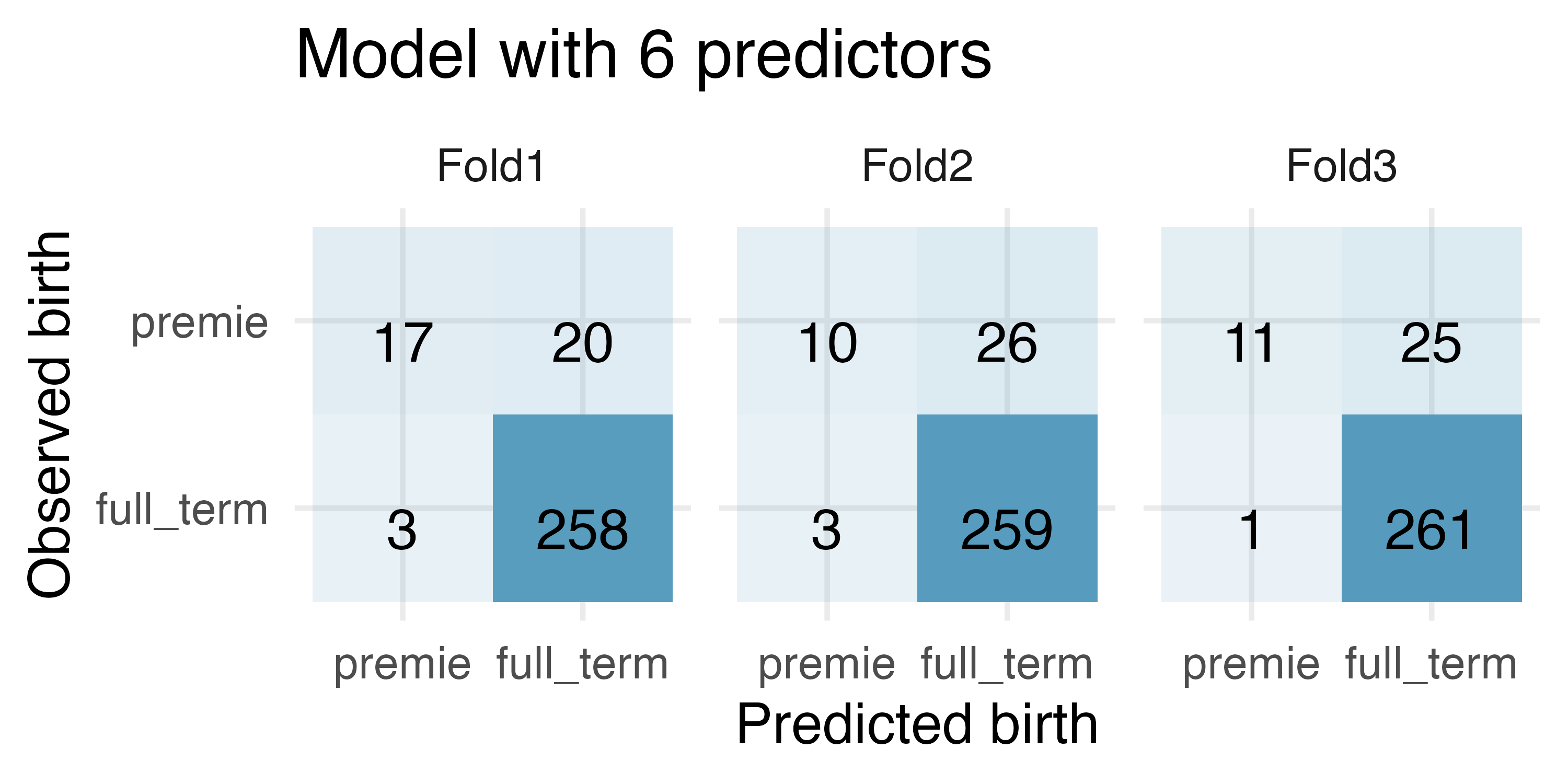
\[ \begin{aligned} \log_e \bigg(\frac{p}{1-p}\bigg) = \beta_0 &+ \beta_1\times \texttt{weight} \\ &+ \beta_2 \times \texttt{mature} \end{aligned} \]
For the model with 6 predictors, how many of the observations were correctly classified? What proportion of the observations were correctly classified?
For the model with 2 predictors, how many of the observations were correctly classified? What proportion of the observations were correctly classified?
If you have to choose between the model with 6 predictors and the model with 2 predictors (for predicting whether a baby will be premature), which model would you choose? Explain.
The
drug_usedata used in this exercise can be found in the openintro R package.↩︎The
sulphinpyrazonedata used in this exercise can be found in the openintro R package.↩︎The
possumdata used in this exercise can be found in the openintro R package.↩︎The
births14data used in this exercise can be found in the openintro R package.↩︎