9 Logistic regression
In this chapter we introduce logistic regression as a tool for building models when there is a categorical response variable with two levels, e.g., yes and no. Logistic regression is a type of generalized linear model (GLM) for response variables where regular multiple regression does not work very well. GLMs can be thought of as a two-stage modeling approach. We first model the response variable using a probability distribution, such as the binomial or Poisson distribution. Second, we model the parameter of the distribution using a collection of predictors and a special form of multiple regression. Ultimately, the application of a GLM will feel very similar to multiple regression, even if some of the details are different.
9.1 Discrimination in hiring
We will consider experiment data from a study that sought to understand the effect of race and sex on job application callback rates (Bertrand and Mullainathan 2003). To evaluate which factors were important, job postings were identified in Boston and Chicago for the study, and researchers created many fake resumes to send off to these jobs to see which would elicit a callback.1 The researchers enumerated important characteristics, such as years of experience and education details, and they used these characteristics to randomly generate fake resumes. Finally, they randomly assigned a name to each resume, where the name would imply the applicant’s sex and race.
The first names that were used and randomly assigned in the experiment were selected so that they would predominantly be recognized as belonging to Black or White individuals; other races were not considered in the study. While no name would definitively be inferred as pertaining to a Black individual or to a White individual, the researchers conducted a survey to check for racial association of the names; names that did not pass the survey check were excluded from usage in the experiment. You can find the full set of names that did pass the survey test and were ultimately used in the study in Table 9.1. For example, Lakisha was a name that their survey indicated would be interpreted as a Black woman, while Greg was a name that would generally be interpreted to be associated with a White male.
| first_name | race | sex | first_name | race | sex | first_name | race | sex |
|---|---|---|---|---|---|---|---|---|
| Aisha | Black | female | Hakim | Black | male | Laurie | White | female |
| Allison | White | female | Jamal | Black | male | Leroy | Black | male |
| Anne | White | female | Jay | White | male | Matthew | White | male |
| Brad | White | male | Jermaine | Black | male | Meredith | White | female |
| Brendan | White | male | Jill | White | female | Neil | White | male |
| Brett | White | male | Kareem | Black | male | Rasheed | Black | male |
| Carrie | White | female | Keisha | Black | female | Sarah | White | female |
| Darnell | Black | male | Kenya | Black | female | Tamika | Black | female |
| Ebony | Black | female | Kristen | White | female | Tanisha | Black | female |
| Emily | White | female | Lakisha | Black | female | Todd | White | male |
| Geoffrey | White | male | Latonya | Black | female | Tremayne | Black | male |
| Greg | White | male | Latoya | Black | female | Tyrone | Black | male |
The response variable of interest is whether there was a callback from the employer for the applicant, and there were 8 attributes that were randomly assigned that we’ll consider, with special interest in the race and sex variables. Race and sex are protected classes in the United States, meaning they are not legally permitted factors for hiring or employment decisions. The full set of attributes considered is provided in Table 26.1.
resume dataset. Many of the variables are indicator variables, meaning they take the value 1 if the specified characteristic is present and 0 otherwise.
| variable | description |
|---|---|
| received_callback | Specifies whether the employer called the applicant following submission of the application for the job. |
| job_city | City where the job was located: Boston or Chicago. |
| college_degree | An indicator for whether the resume listed a college degree. |
| years_experience | Number of years of experience listed on the resume. |
| honors | Indicator for the resume listing some sort of honors, e.g. employee of the month. |
| military | Indicator for if the resume listed any military experience. |
| has_email_address | Indicator for if the resume listed an email address for the applicant. |
| race | Race of the applicant, implied by their first name listed on the resume. |
| sex | Sex of the applicant (limited to only man and woman), implied by the first name listed on the resume. |
All of the attributes listed on each resume were randomly assigned, which means that no attributes that might be favorable or detrimental to employment would favor one demographic over another on these resumes. Importantly, due to the experimental nature of the study, we can infer causation between these variables and the callback rate, if substantial differences are found. Our analysis will allow us to compare the practical importance of each of the variables relative to each other.
9.2 Modelling the probability of an event
Logistic regression is a generalized linear model where the outcome is a two-level categorical variable. The outcome, \(Y_i\), takes the value 1 (in our application, the outcome represents a callback for the resume) with probability \(p_i\) and the value 0 with probability \(1 - p_i\). Because each observation has a slightly different context, e.g., different education level or a different number of years of experience, the probability \(p_i\) will differ for each observation. Ultimately, it is the probability of the outcome taking the value 1 (i.e., being a “success”) that we model in relation to the predictor variables: we will examine which resume characteristics correspond to higher or lower callback rates.
Notation for a logistic regression model.
The outcome variable for a GLM is denoted by \(Y_i\), where the index \(i\) is used to represent observation \(i\). In the resume application, \(Y_i\) will be used to represent whether resume \(i\) received a callback (\(Y_i=1\)) or not (\(Y_i=0\)).
The predictor variables are represented as follows: \(x_{1,i}\) is the value of variable 1 for observation \(i\), \(x_{2,i}\) is the value of variable 2 for observation \(i\), and so on.
\[ transformation(p_i) = \beta_0 + \beta_1 x_{1,i} + \beta_2 x_{2,i} + \cdots + \beta_k x_{k,i} \]
We want to choose a transformation in the equation that makes practical and mathematical sense. For example, we want a transformation that makes the range of possibilities on the left hand side of the equation equal to the range of possibilities for the right hand side; if there was no transformation in the equation, the left hand side could only take values between 0 and 1, but the right hand side could take values well outside of the range from 0 to 1.
A common transformation for \(p_i\) is the logit transformation, which may be written as
\[ logit(p_i) = \log_{e}\left( \frac{p_i}{1-p_i} \right) \]
The logit transformation is shown in Figure 9.1. Below, we rewrite the equation relating \(Y_i\) to its predictors using the logit transformation of \(p_i\):
\[ \log_{e}\left( \frac{p_i}{1-p_i} \right) = \beta_0 + \beta_1 x_{1,i} + \beta_2 x_{2,i} + \cdots + \beta_k x_{k,i} \]
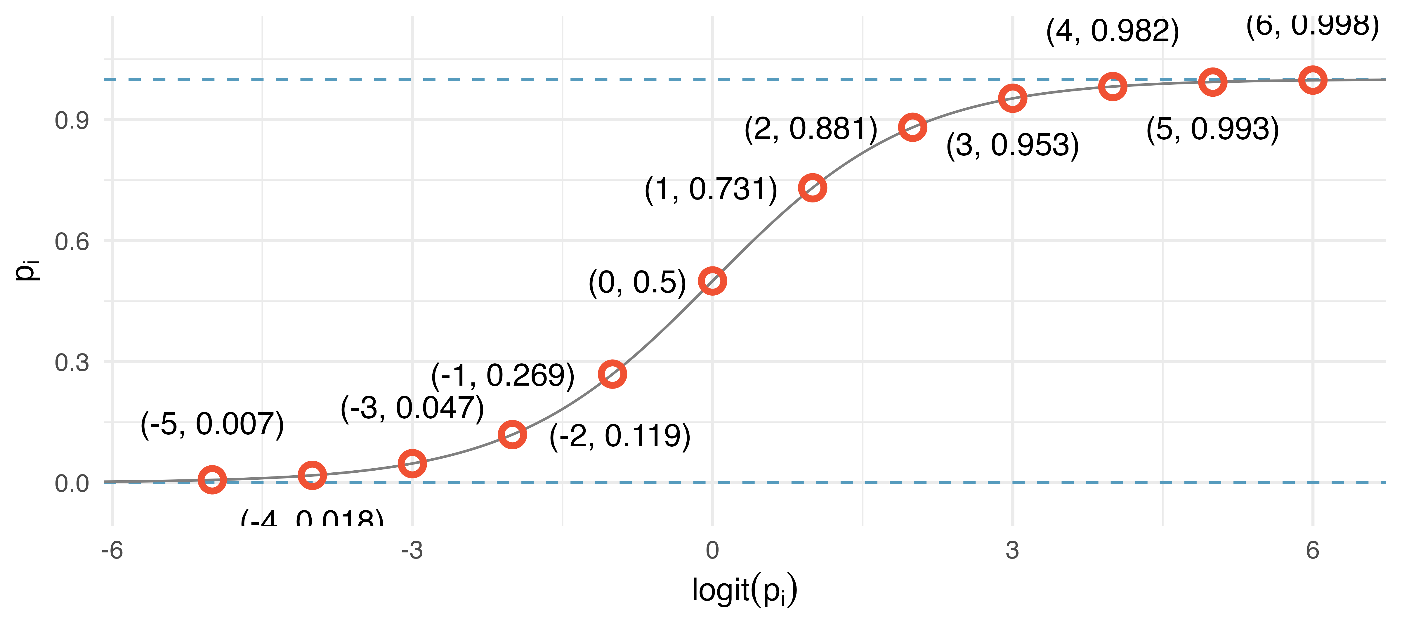
In our resume example, there are 8 predictor variables, so \(k = 8\). While the precise choice of a logit function isn’t intuitive, it is based on theory that underpins generalized linear models, which is beyond the scope of this book. Fortunately, once we fit a model using software, it will start to feel like we are back in the multiple regression context, even if the interpretation of the coefficients is more complex.
To convert from values on the logistic regression scale to the probability scale, we need to back transform and then solve for \(p_i\):
\[ \begin{aligned} \log_{e}\left( \frac{p_i}{1-p_i} \right) &= \beta_0 + \beta_1 x_{1,i} + \cdots + \beta_k x_{k,i} \\ \frac{p_i}{1-p_i} &= e^{\beta_0 + \beta_1 x_{1,i} + \cdots + \beta_k x_{k,i}} \\ p_i &= \left( 1 - p_i \right) e^{\beta_0 + \beta_1 x_{1,i} + \cdots + \beta_k x_{k,i}} \\ p_i &= e^{\beta_0 + \beta_1 x_{1,i} + \cdots + \beta_k x_{k,i}} - p_i \times e^{\beta_0 + \beta_1 x_{1,i} + \cdots + \beta_k x_{k,i}} \\ p_i + p_i \text{ } e^{\beta_0 + \beta_1 x_{1,i} + \cdots + \beta_k x_{k,i}} &= e^{\beta_0 + \beta_1 x_{1,i} + \cdots + \beta_k x_{k,i}} \\ p_i(1 + e^{\beta_0 + \beta_1 x_{1,i} + \cdots + \beta_k x_{k,i}}) &= e^{\beta_0 + \beta_1 x_{1,i} + \cdots + \beta_k x_{k,i}} \\ p_i &= \frac{e^{\beta_0 + \beta_1 x_{1,i} + \cdots + \beta_k x_{k,i}}}{1 + e^{\beta_0 + \beta_1 x_{1,i} + \cdots + \beta_k x_{k,i}}} \end{aligned} \]
As with most applied data problems, we substitute in the point estimates (the observed \(b_i\)) to calculate relevant probabilities.
We start by fitting a model with a single predictor: honors. This variable indicates whether the applicant had any type of honors listed on their resume, such as employee of the month. A logistic regression model was fit using statistical software and the following model was found:
\[\log_e \left( \frac{\widehat{p}_i}{1-\widehat{p}_i} \right) = -2.4998 + 0.8668 \times {\texttt{honors}}\]
If a resume is randomly selected from the study and it does not have any honors listed, what is the probability it resulted in a callback?
What would the probability be if the resume did list some honors?
If a randomly chosen resume from those sent out is considered, and it does not list honors, then
honorstakes the value of 0 and the right side of the model equation equals -2.4998. Solving for \(p_i\): \(\frac{e^{-2.4998}}{1 + e^{-2.4998}} = 0.076\). Just as we labeled a fitted value of \(y_i\) with a “hat” in single-variable and multiple regression, we do the same for this probability: \(\hat{p}_i = 0.076{}\).If the resume had listed some honors, then the right side of the model equation is \(-2.4998 + 0.8668 \times 1 = -1.6330\), which corresponds to a probability \(\hat{p}_i = 0.163\). Notice that we could examine -2.4998 and -1.6330 in Figure 9.1 to estimate the probability before formally calculating the value.
While knowing whether a resume listed honors provides some signal when predicting whether the employer would call, we would like to account for many different variables at once to understand how each of the different resume characteristics affected the chance of a callback.
9.3 Logistic model with many variables
We used statistical software to fit the logistic regression model with all 8 predictors described in Table 26.1. Like multiple regression, the result may be presented in a summary table, which is shown in Table 9.3.
| term | estimate | std.error | statistic | p.value |
|---|---|---|---|---|
| (Intercept) | -2.66 | 0.18 | -14.64 | <0.0001 |
| job_cityChicago | -0.44 | 0.11 | -3.85 | 1e-04 |
| college_degree1 | -0.07 | 0.12 | -0.55 | 0.5821 |
| years_experience | 0.02 | 0.01 | 1.96 | 0.0503 |
| honors1 | 0.77 | 0.19 | 4.14 | <0.0001 |
| military1 | -0.34 | 0.22 | -1.59 | 0.1127 |
| has_email_address1 | 0.22 | 0.11 | 1.93 | 0.0541 |
| raceWhite | 0.44 | 0.11 | 4.10 | <0.0001 |
| sexman | -0.18 | 0.14 | -1.32 | 0.1863 |
Just like multiple regression, we could trim some variables from the model. Here we’ll use a statistic called Akaike information criterion (AIC), which is analogous to how we used adjusted \(R^2\) in multiple regression. AIC is a popular model selection method used in many disciplines, and is praised for its emphasis on model uncertainty and parsimony. AIC selects a “best” model by ranking models from best to worst according to their AIC values. In the calculation of a model’s AIC, a penalty is given for including additional variables. The penalty for added model complexity attempts to strike a balance between underfitting (too few variables in the model) and overfitting (too many variables in the model). When using AIC for model selection, models with a lower AIC value are considered to be “better.” Remember that when using adjusted \(R^2\) we select models with higher values instead. It is important to note that AIC provides information about the quality of a model relative to other models, but does not provide information about the overall quality of a model.
Table 9.4 provides the AIC and the number of observations used to fit the model. We also know from Table 9.3 that eight variables (with nine coefficients, including the intercept) were fit.
| AIC | number_observations |
|---|---|
| 2677 | 4870 |
We will look for models with a lower AIC using a backward elimination strategy. Table 9.5 provides the AIC values for the model with variables as given in Table 9.6. Notice that the same number of observations are used, but one fewer variable (college_degree is dropped from the model).
college_degree.
| AIC | number_observations |
|---|---|
| 2676 | 4870 |
After using the AIC criteria, the variable college_degree is eliminated (the AIC value without college_degree is smaller than the AIC value on the full model), giving the model summarized in Table 9.6 with fewer variables, which is what we’ll rely on for the remainder of the section.
college_degree has been dropped from the model.
| term | estimate | std.error | statistic | p.value |
|---|---|---|---|---|
| (Intercept) | -2.72 | 0.16 | -17.51 | <0.0001 |
| job_cityChicago | -0.44 | 0.11 | -3.83 | 1e-04 |
| years_experience | 0.02 | 0.01 | 2.02 | 0.043 |
| honors1 | 0.76 | 0.19 | 4.12 | <0.0001 |
| military1 | -0.34 | 0.22 | -1.60 | 0.1105 |
| has_email_address1 | 0.22 | 0.11 | 1.97 | 0.0494 |
| raceWhite | 0.44 | 0.11 | 4.10 | <0.0001 |
| sexman | -0.20 | 0.14 | -1.45 | 0.1473 |
The race variable had taken only two levels: Black and White. Based on the model results, what does the coefficient of the race variable say about callback decisions?
The coefficient shown corresponds to the level of White, and it is positive. The positive coefficient reflects a positive gain in callback rate for resumes where the candidate’s first name implied they were White. The model results suggest that prospective employers favor resumes where the first name is typically interpreted to be White.
The coefficient of \(\texttt{race}_{\texttt{White}}\) in the full model in Table 9.3, is nearly identical to the model shown in Table 9.6. The predictors in the experiment were thoughtfully laid out so that the coefficient estimates would typically not be much influenced by which other predictors were in the model, which aligned with the motivation of the study to tease out which effects were important to getting a callback. In most observational data, it’s common for point estimates to change a little, and sometimes a lot, depending on which other variables are included in the model.
Use the model summarized in Table 9.6 to estimate the probability of receiving a callback for a job in Chicago where the candidate lists 14 years experience, no honors, no military experience, includes an email address, and has a first name that implies they are a White male.
We can start by writing out the equation using the coefficients from the model:
\[ \begin{aligned} log_e \left(\frac{\widehat{p}}{1 - \widehat{p}}\right) = -2.7162 &- 0.4364 \times \texttt{job\_city}_{\texttt{Chicago}} + 0.0206 \times \texttt{years\_experience} \\ &+ 0.7634 \times \texttt{honors} - 0.3443 \times \texttt{military} + 0.2221 \times \texttt{email} \\ &+ 0.4429 \times \texttt{race}_{\texttt{White}} - 0.1959 \times \texttt{sex}_{\texttt{man}} \end{aligned} \]
Now we can add in the corresponding values of each variable for the individual of interest:
\[ \begin{aligned} log_e \left(\frac{\widehat{p}}{1 - \widehat{p}}\right) = - 2.7162 &- 0.4364 \times 1 + 0.0206 \times 14 \\ &+ 0.7634 \times 0 - 0.3443 \times 0 + 0.2221 \times 1 \\ &+ 0.4429 \times 1 - 0.1959 \times 1 = - 2.3955 \end{aligned} \]
We can now back-solve for \(\widehat{p}\): the chance such an individual will receive a callback is about \(\frac{e^{-2.3955}}{1 + e^{-2.3955}} = 0.0835.\)
Compute the probability of a callback for an individual with a name commonly inferred to be from a Black male but who otherwise has the same characteristics as the one described in the previous example.
We can complete the same steps for an individual with the same characteristics who is Black, where the only difference in the calculation is that the indicator variable \(\texttt{race}_{\texttt{White}}\) will take a value of 0. Doing so yields a probability of 0.0553. Let’s compare the results with those of the previous example.
In practical terms, an individual perceived as White based on their first name would need to apply to \(\frac{1}{0.0835} \approx 12\) jobs on average to receive a callback, while an individual perceived as Black based on their first name would need to apply to \(\frac{1}{0.0553} \approx 18\) jobs on average to receive a callback. That is, applicants who are perceived as Black need to apply to 50% more employers to receive a callback than someone who is perceived as White based on their first name for jobs like those in the study.
What we have quantified in the current section is alarming and disturbing. However, one aspect that makes the racism so difficult to address is that the experiment, as well-designed as it is, cannot send us much signal about which employers are discriminating. It is only possible to say that discrimination is happening, even if we cannot say which particular callbacks — or non-callbacks — represent discrimination. Finding strong evidence of racism for individual cases is a persistent challenge in enforcing anti-discrimination laws.
9.4 Groups of different sizes
Any form of discrimination is concerning, which is why we decided it was so important to discuss the topic using data. The resume study also only examined discrimination in a single aspect: whether a prospective employer would call a candidate who submitted their resume. There was a 50% higher barrier for resumes simply when the candidate had a first name that was perceived to be of a Black individual. It’s unlikely that discrimination would stop there.
Let’s consider a sex-imbalanced company that consists of 20% women and 80% men, and we’ll suppose that the company is very large, consisting of perhaps 20,000 employees. (A more deliberate example would include more inclusive gender identities.) Suppose when someone goes up for promotion at the company, 5 of their colleagues are randomly chosen to provide feedback on their work.
Now let’s imagine that 10% of the people in the company are prejudiced against the other sex. That is, 10% of men are prejudiced against women, and similarly, 10% of women are prejudiced against men. Who is discriminated against more at the company, men or women?
Let’s suppose we took 100 men who have gone up for promotion in the past few years. For these men, \(5 \times 100 = 500\) random colleagues will be tapped for their feedback, of which about 20% will be women (100 women). Of these 100 women, 10 are expected to be biased against the man they are reviewing. Then, of the 500 colleagues reviewing them, men will experience discrimination by about 2% of their colleagues when they go up for promotion.
Let’s do a similar calculation for 100 women who have gone up for promotion in the last few years. They will also have 500 random colleagues providing feedback, of which about 400 (80%) will be men. Of these 400 men, about 40 (10%) hold a bias against women. Of the 500 colleagues providing feedback on the promotion packet for these women, 8% of the colleagues hold a bias against the women.
The example highlights something profound: even in a hypothetical setting where each demographic has the same degree of prejudice against the other demographic, the smaller group experiences the negative effects more frequently. Additionally, if we would complete a handful of examples like the one above with different numbers, we would learn that the greater the imbalance in the population groups, the more the smaller group is disproportionately impacted.2
Of course, there are other considerable real-world omissions from the hypothetical example. For example, studies have found instances where people from an oppressed group also discriminate against others within their own oppressed group. As another example, there are also instances where a majority group can be oppressed, with apartheid in South Africa being one such historic example. Ultimately, discrimination is complex, and there are many factors at play beyond the mathematics property we observed in the previous example.
We close the chapter on the serious topic of discrimination, and we hope it inspires you to think about the power of reasoning with data. Whether it is with a formal statistical model or by using critical thinking skills to structure a problem, we hope the ideas you have learned will help you do more and do better in life.
9.5 Chapter review
9.5.1 Summary
Logistic and linear regression models have many similarities. The strongest of which is the linear combination of the explanatory variables which is used to form predictions related to the response variable. However, with logistic regression, the response variable is binary and therefore a prediction is given on the probability of a successful event. Logistic model fit and variable selection can be carried out in similar ways as multiple linear regression.
9.5.2 Terms
The terms introduced in this chapter are presented in Table 9.7. If you’re not sure what some of these terms mean, we recommend you go back in the text and review their definitions. You should be able to easily spot them as bolded text.
| AIC | logistic regression | transformation |
| Akaike information criterion | logit transformation | |
| generalized linear model | probability of an event |
9.6 Exercises
Answers to odd-numbered exercises can be found in Appendix A.9.
-
True / False. Determine which of the following statements are true and false. For each statement that is false, explain why it is false.
In logistic regression we fit a line to model the relationship between the predictor(s) and the binary outcome.
In logistic regression, we expect the residuals to be even scattered on either side of zero, just like with linear regression.
In logistic regression, the outcome variable is binary but the predictor variable(s) can be either binary or continuous.
-
Logistic regression fact checking. Determine which of the following statements are true and false. For each statement that is false, explain why it is false.
Suppose we consider the first two observations based on a logistic regression model, where the first variable in observation 1 takes a value of \(x_1 = 6\) and observation 2 has \(x_1 = 4\). Suppose we realized we made an error for these two observations, and the first observation was actually \(x_1 = 7\) (instead of 6) and the second observation actually had \(x_1 = 5\) (instead of 4). Then the predicted probability from the logistic regression model would increase the same amount for each observation after we correct these variables.
When using a logistic regression model, it is impossible for the model to predict a probability that is negative or a probability that is greater than 1.
Because logistic regression predicts probabilities of outcomes, observations used to build a logistic regression model need not be independent.
When fitting logistic regression, we typically complete model selection using adjusted \(R^2\).
-
Possum classification, comparing models. The common brushtail possum of the Australia region is a bit cuter than its distant cousin, the American opossum (see Figure 7.4). We consider 104 brushtail possums from two regions in Australia, where the possums may be considered a random sample from the population. The first region is Victoria, which is in the eastern half of Australia and traverses the southern coast. The second region consists of New South Wales and Queensland, which make up eastern and northeastern Australia.3
We use logistic regression to differentiate between possums in these two regions. The outcome variable, called
pop, takes value 1 when a possum is from Victoria and 0 when it is from New South Wales or Queensland. We consider five predictors:sex(an indicator for a possum being male),head_l(head length),skull_w(skull width),total_l(total length), andtail_l(tail length). Each variable is summarized in a histogram. The full logistic regression model and a reduced model after variable selection are summarized in the tables below.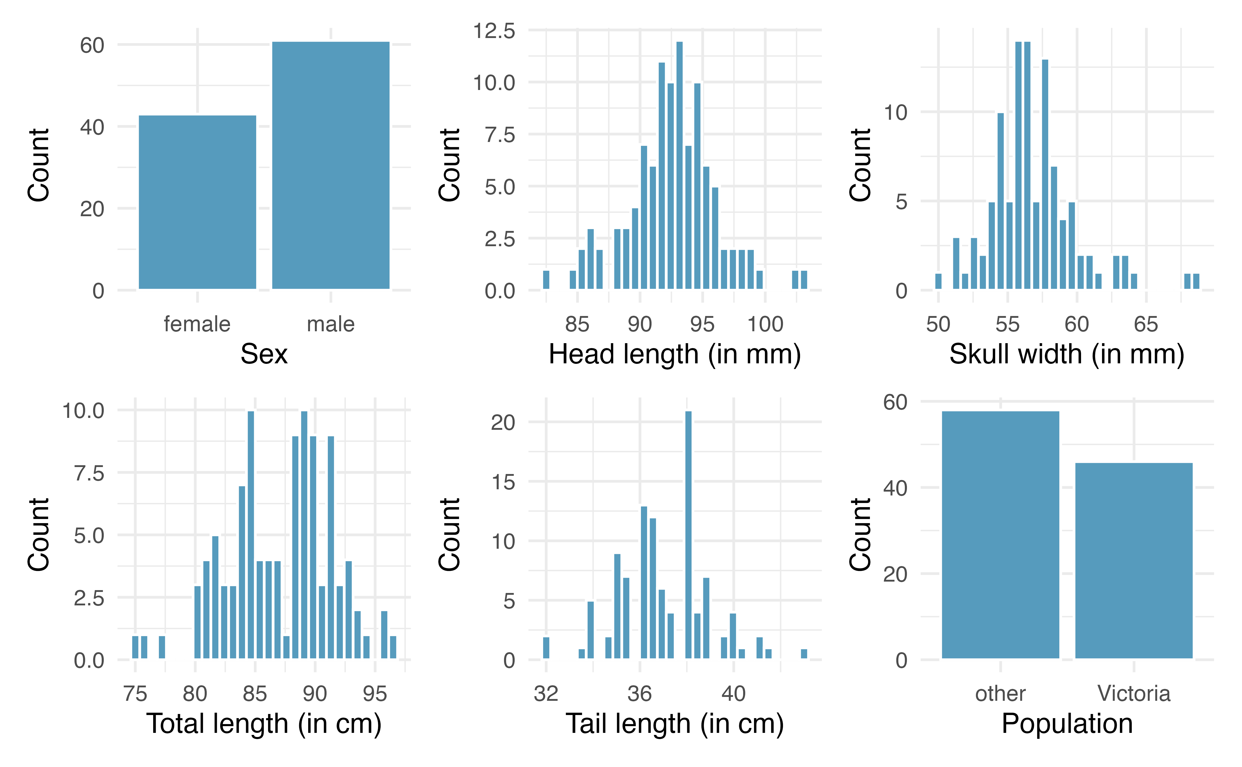
term estimate std.error statistic p.value (Intercept) 39.23 11.54 3.40 7e-04 sexmale -1.24 0.67 -1.86 0.0632 head_l -0.16 0.14 -1.16 0.248 skull_w -0.20 0.13 -1.52 0.1294 total_l 0.65 0.15 4.24 <0.0001 tail_l -1.87 0.37 -5.00 <0.0001 term estimate std.error statistic p.value (Intercept) 33.51 9.91 3.38 7e-04 sexmale -1.42 0.65 -2.20 0.0278 skull_w -0.28 0.12 -2.27 0.0231 total_l 0.57 0.13 4.30 <0.0001 tail_l -1.81 0.36 -5.02 <0.0001 Examine each of the predictors given by the individual graphs. Are there any outliers that are likely to have a very large influence on the logistic regression model?
Two models are provided above for predicting the region of the possum. (In Chapter 26 we will cover a method for deciding between the models based on p-values.) The first model includes
head_land the second model does not. Explain why the remaining estimates (model coefficients) change between the two models.
-
Challenger disaster and model building. On January 28, 1986, a routine launch was anticipated for the Challenger space shuttle. Seventy-three seconds into the flight, disaster happened: the shuttle broke apart, killing all seven crew members on board. An investigation into the cause of the disaster focused on a critical seal called an O-ring, and it is believed that damage to these O-rings during a shuttle launch may be related to the ambient temperature during the launch. The table below summarizes observational data on O-rings for 23 shuttle missions, where the mission order is based on the temperature at the time of the launch.
temperaturegives the temperature in Fahrenheit,damagedrepresents the number of damaged O-rings, andundamagedrepresents the number of O-rings that were not damaged.4mission 1 2 3 4 5 6 7 8 9 10 11 12 temperature 53 57 58 63 66 67 67 67 68 69 70 70 damaged 5 1 1 1 0 0 0 0 0 0 1 0 undamaged 1 5 5 5 6 6 6 6 6 6 5 6 mission 13 14 15 16 17 18 19 20 21 22 23 temperature 70 70 72 73 75 75 76 76 78 79 81 damaged 1 0 0 0 0 1 0 0 0 0 0 undamaged 5 6 6 6 6 5 6 6 6 6 6 term estimate std.error statistic p.value (Intercept) 11.66 3.30 3.54 4e-04 temperature -0.22 0.05 -4.07 <0.0001 Each column of the table above represents a different shuttle mission. Examine these data and describe what you observe with respect to the relationship between temperatures and damaged O-rings.
Failures have been coded as 1 for a damaged O-ring and 0 for an undamaged O-ring, and a logistic regression model was fit to these data. The regression output for this model is given above. Describe the key components of the output in words.
Write out the logistic model using the point estimates of the model parameters.
Based on the model, do you think concerns regarding O-rings are justified? Explain.
-
Possum classification, prediction. A logistic regression model was proposed for classifying common brushtail possums into their two regions. The outcome variable took value 1 if the possum was from Victoria and 0 otherwise.
term estimate std.error statistic p.value (Intercept) 33.51 9.91 3.38 7e-04 sexmale -1.42 0.65 -2.20 0.0278 skull_w -0.28 0.12 -2.27 0.0231 total_l 0.57 0.13 4.30 <0.0001 tail_l -1.81 0.36 -5.02 <0.0001 Write out the form of the model. Also identify which of the variables are positively associated with the outcome of living in Victoria, when controlling for other variables.
Suppose we see a brushtail possum at a zoo in the US, and a sign says the possum had been captured in the wild in Australia, but it doesn’t say which part of Australia. However, the sign does indicate that the possum is male, its skull is about 63 mm wide, its tail is 37 cm long, and its total length is 83 cm. What is the reduced model’s computed probability that this possum is from Victoria? How confident are you in the model’s accuracy of this probability calculation?
-
Challenger disaster and prediction. On January 28, 1986, a routine launch was anticipated for the Challenger space shuttle. Seventy-three seconds into the flight, disaster happened: the shuttle broke apart, killing all seven crew members on board. An investigation into the cause of the disaster focused on a critical seal called an O-ring, and it is believed that damage to these O-rings during a shuttle launch may be related to the ambient temperature during the launch. The investigation found that the ambient temperature at the time of the shuttle launch was closely related to the damage of O-rings, which are a critical component of the shuttle.
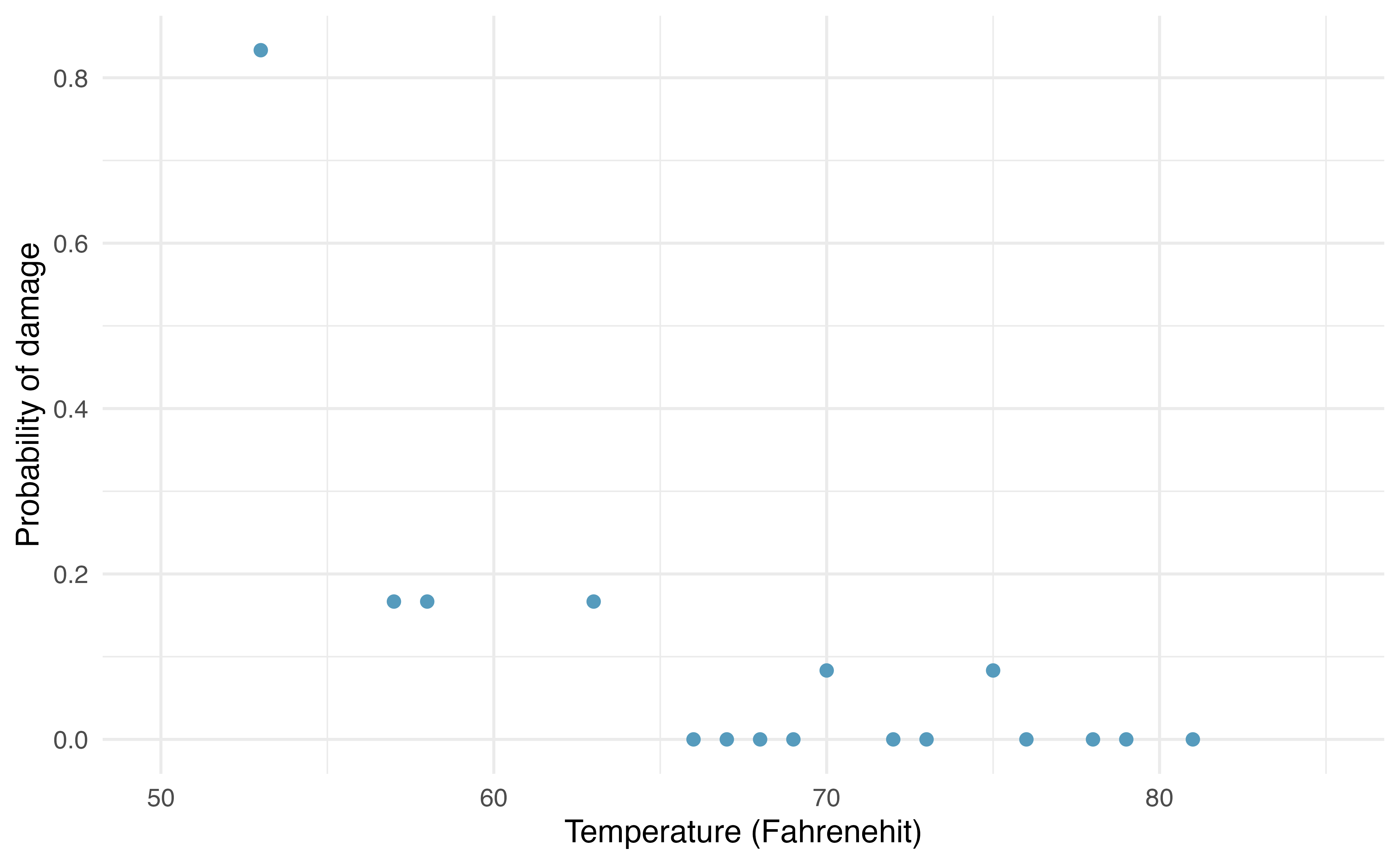
- The data provided in the previous exercise are shown in the plot. The logistic model fit to these data may be written as
\[\log\left( \frac{\hat{p}}{1 - \hat{p}} \right) = 11.6630 - 0.2162\times \texttt{temperature}\]
where \(\hat{p}\) is the model-estimated probability that an O-ring will become damaged. Use the model to calculate the probability that an O-ring will become damaged at each of the following ambient temperatures: 51, 53, and 55 degrees Fahrenheit. The model-estimated probabilities for several additional ambient temperatures are provided below, where subscripts indicate the temperature:
\[ \begin{aligned} &\hat{p}_{57} = 0.341 && \hat{p}_{59} = 0.251 && \hat{p}_{61} = 0.179 && \hat{p}_{63} = 0.124 \\ &\hat{p}_{65} = 0.084 && \hat{p}_{67} = 0.056 && \hat{p}_{69} = 0.037 && \hat{p}_{71} = 0.024 \end{aligned} \]
Add the model-estimated probabilities from part (a) on the plot, then connect these dots using a smooth curve to represent the model-estimated probabilities.
Describe any concerns you may have regarding applying logistic regression in this application, and note any assumptions that are required to accept the model’s validity.
-
Spam filtering, model selection. Spam filters are built on principles similar to those used in logistic regression. Using characteristics of individual emails, we fit a probability that each message is spam or not spam. We have several email variables for this problem, and we won’t describe what each variable means here for the sake of brevity, but each is either a numerical or indicator variable.5
term estimate std.error statistic p.value (Intercept) -0.69 0.09 -7.42 <0.0001 to_multiple1 -2.82 0.31 -9.05 <0.0001 cc 0.03 0.02 1.41 0.1585 attach 0.28 0.08 3.44 6e-04 dollar -0.08 0.02 -3.45 6e-04 winneryes 1.72 0.34 5.09 <0.0001 inherit 0.32 0.15 2.10 0.0355 password -0.79 0.30 -2.64 0.0083 format1 -1.50 0.13 -12.01 <0.0001 re_subj1 -1.92 0.38 -5.10 <0.0001 exclaim_subj 0.26 0.23 1.14 0.2531 sent_email1 -16.67 293.19 -0.06 0.9547 The AIC of the full model is 1863.5. We remove each variable one by one, refit the model, and record the updated AIC.
- For variable selection, we fit the full model, which includes all variables, and then we also fit each model where we’ve dropped exactly one of the variables. In each of these reduced models, the AIC value for the model is reported below. Based on these results, which variable, if any, should we drop as part of model selection? Explain.
- None Dropped: 1863.5
- Drop
to_multiple: 2023.5 - Drop
cc: 1863.2 - Drop
attach: 1871.9 - Drop
dollar: 1879.7 - Drop
winner: 1885
- Drop
inherit: 1865.5 - Drop
password: 1879.3 - Drop
format: 2008.9 - Drop
re_subj: 1904.6 - Drop
exclaim_subj: 1862.8 - Drop
sent_email: 1958.2
- Consider the subsequent model selection stage (where the variable from part (a) has been removed, and we are considering removal of a second variable). Here again we’ve computed the AIC for each leave-one-variable-out model. Based on the results, which variable, if any, should we drop as part of model selection? Explain.
- None dropped: 1862.8
- Drop
to_multiple: 2021.5 - Drop
cc: 1862.4 - Drop
attach: 1871.2 - Drop
dollar: 1877.8 - Drop
winner: 1885.2
- Drop
inherit: 1864.8 - Drop
password: 1878.4 - Drop
format: 2007 - Drop
re_subj: 1904.3 - Drop
sent_email: 1957.3
- Consider one more step in the process. Here again we’ve computed the AIC for each leave-one-variable-out model. Based on the results, which variable, if any, should we drop as part of model selection? Explain.
- None Dropped: 1862.4
- Drop
to_multiple: 2019.6 - Drop
attach: 1871.2 - Drop
dollar: 1877.7 - Drop
winner: 1885
- Drop
inherit: 1864.5 - Drop
password: 1878.2 - Drop
format: 2007.4 - Drop
re_subj: 1902.9 - Drop
sent_email: 1957.6
-
Spam filtering, prediction. Recall running a logistic regression to aid in spam classification for individual emails. In this exercise, we’ve taken a small set of the variables and fit a logistic model with the following output:
term estimate std.error statistic p.value (Intercept) -0.81 0.09 -9.34 <0.0001 to_multiple1 -2.64 0.30 -8.68 <0.0001 winneryes 1.63 0.32 5.11 <0.0001 format1 -1.59 0.12 -13.28 <0.0001 re_subj1 -3.05 0.36 -8.40 <0.0001 Write down the model using the coefficients from the model fit.
Suppose we have an observation where \(\texttt{to\_multiple} = 0\), \(\texttt{winner}= 1\), \(\texttt{format} = 0\), and \(\texttt{re\_subj} = 0\). What is the predicted probability that this message is spam?
Put yourself in the shoes of a data scientist working on a spam filter. For a given message, how high must the probability a message is spam be before you think it would be reasonable to put it in a spambox (which the user is unlikely to check)? What tradeoffs might you consider? Any ideas about how you might make your spam-filtering system even better from the perspective of someone using your email service?
-
Possum classification, model selection via AIC. A logistic regression model was proposed for classifying common brushtail possums into their two regions. The outcome variable took value 1 if the possum was from Victoria and 0 otherwise.
We use logistic regression to classify the 104 possums in our dataset in these two regions. The outcome variable, called
pop, takes value 1 when the possum is from Victoria and 0 when it is from New South Wales or Queensland. We consider five predictors:sex(an indicator for a possum being male),head_l(head length),skull_w(skull width),total_l(total length), andtail_l(tail length).A summary of the three models we fit and their AIC values are given below:
formula AIC sex + head_l + skull_w + total_l + tail_l 84.2 sex + skull_w + total_l + tail_l 83.5 sex + head_l + total_l + tail_l 84.7 Using the AIC metric, which of the three models would be best to report?
If, for example, the AIC is virtually equivalent for two models that have differing numbers of variables, which model would be prefered: the model with more variables or the model with fewer variables? Explain.
- Model selection. An important aspect of building a logistic regression model is figuring out which variables to include in the model. In Chapter 9 we covered using AIC to choose between variable subsets. In Chapter 26 we will cover using something called p-values to choose between variables subsets. Alternatively, you might hope that a model gave the smallest number of false positives, the smallest number of false negatives, or the highest overall accuracy. If different criteria produce outcomes of different variable subsets for the final model, how might you decide which model to put forward? (Hint: There is no single correct answer to this question.)
We did omit discussion of some structure in the data for the analysis presented: the experiment design included blocking, where typically four resumes were sent to each job: one for each inferred race/sex combination (as inferred based on the first name). We did not worry about the blocking aspect, since accounting for the blocking would reduce the standard error without notably changing the point estimates for the
raceandsexvariables versus the analysis performed in the section. That is, the most interesting conclusions in the study are unaffected even when completing a more sophisticated analysis.↩︎If a proportion \(p\) of a company are women and the rest of the company consists of men, then under the hypothetical situation the ratio of rates of discrimination against women versus men would be given by \((1 - p) / p,\) a ratio that is always greater than 1 when \(p < 0.5\).↩︎
The
possumdata used in this exercise can be found in the openintro R package.↩︎The
oringsdata used in this exercise can be found in the openintro R package.↩︎The
emaildata used in this exercise can be found in the openintro R package.↩︎