8 Linear regression with multiple predictors
Building on the ideas of one predictor variable in a linear regression model (from Chapter 7), a multiple linear regression model is now fit to two or more predictor variables. By considering how different explanatory variables interact, we can uncover complicated relationships between the predictor variables and the response variable. One challenge to working with multiple variables is that it is sometimes difficult to know which variables are most important to include in the model. Model building is an extensive topic, and we scratch the surface here by defining and utilizing the adjusted \(R^2\) value.
Multiple regression extends single predictor variable regression to the case that still has one response but many predictors (denoted \(x_1\), \(x_2\), \(x_3\), …). The method is motivated by scenarios where many variables may be simultaneously connected to an output.
We will consider data about loans from the peer-to-peer lender, Lending Club, which is a dataset we first encountered in Chapter 1. The loan data includes terms of the loan as well as information about the borrower. The outcome variable we would like to better understand is the interest rate assigned to the loan. For instance, all other characteristics held constant, does it matter how much debt someone already has? Does it matter if their income has been verified? Multiple regression will help us answer these and other questions.
The dataset includes information on 10000 loans, and we’ll be looking at a subset of the available variables, some of which will be new from those we saw in earlier chapters. The first six observations in the dataset are shown in Table 8.1, and descriptions for each variable are shown in Table 8.2. Notice that the past bankruptcy variable (bankruptcy) is an indicator variable, where it takes the value 1 if the borrower had a past bankruptcy in their record and 0 if not. Using an indicator variable in place of a category name allows for these variables to be directly used in regression. Two of the other variables are categorical (verified_income and issue_month), each of which can take one of a few different non-numerical values; we’ll discuss how these are handled in the model in Section 8.1.
The loans_full_schema data can be found in the openintro R package. Based on the data in this dataset we have created two new variables: credit_util which is calculated as the total credit utilized divided by the total credit limit and bankruptcy which turns the number of bankruptcies to an indicator variable (0 for no bankruptcies and 1 for at least 1 bankruptcy). We will refer to this modified dataset as loans.
loans dataset.
| interest_rate | verified_income | debt_to_income | credit_util | bankruptcy | term | credit_checks | issue_month |
|---|---|---|---|---|---|---|---|
| 14.07 | Verified | 18.01 | 0.548 | 0 | 60 | 6 | Mar-2018 |
| 12.61 | Not Verified | 5.04 | 0.150 | 1 | 36 | 1 | Feb-2018 |
| 17.09 | Source Verified | 21.15 | 0.661 | 0 | 36 | 4 | Feb-2018 |
| 6.72 | Not Verified | 10.16 | 0.197 | 0 | 36 | 0 | Jan-2018 |
| 14.07 | Verified | 57.96 | 0.755 | 0 | 36 | 7 | Mar-2018 |
| 6.72 | Not Verified | 6.46 | 0.093 | 0 | 36 | 6 | Jan-2018 |
loans dataset.
| Variable | Description |
|---|---|
| interest_rate | Interest rate on the loan, in an annual percentage. |
| verified_income | Categorical variable describing whether the borrower's income source and amount have been verified, with levels Verified (source and amount verified), Source Verified (source only verified), and Not Verified. |
| debt_to_income | Debt-to-income ratio, which is the percentage of total debt of the borrower divided by their total income. |
| credit_util | Of all the credit available to the borrower, what fraction are they utilizing. For example, the credit utilization on a credit card would be the card's balance divided by the card's credit limit. |
| bankruptcy | An indicator variable for whether the borrower has a past bankruptcy in their record. This variable takes a value of `1` if the answer is *yes* and `0` if the answer is *no*. |
| term | The length of the loan, in months. |
| issue_month | The month and year the loan was issued, which for these loans is always during the first quarter of 2018. |
| credit_checks | Number of credit checks in the last 12 months. For example, when filing an application for a credit card, it is common for the company receiving the application to run a credit check. |
8.1 Indicator and categorical predictors
Let’s start by fitting a linear regression model for interest rate with a single predictor indicating whether a person has a bankruptcy in their record:
\[ \widehat{\texttt{interest\_rate}} = 12.34 + 0.74 \times \texttt{bankruptcy} \]
Results of this model are shown in Table 8.3.
interest_rate based on whether the borrower has a bankruptcy in their record. Degrees of freedom for this model is 9998.
| term | estimate | std.error | statistic | p.value |
|---|---|---|---|---|
| (Intercept) | 12.34 | 0.05 | 231.49 | <0.0001 |
| bankruptcy1 | 0.74 | 0.15 | 4.82 | <0.0001 |
Interpret the coefficient for the past bankruptcy variable in the model.
The variable takes one of two values: 1 when the borrower has a bankruptcy in their history and 0 otherwise. A slope of 0.74 means that the model predicts a 0.74% higher interest rate for those borrowers with a bankruptcy in their record. (See Section 7.2.6 for a review of the interpretation for two-level categorical predictor variables.)
Suppose we had fit a model using a 3-level categorical variable, such as verified_income. The output from software is shown in Table 8.4. This regression output provides multiple rows for the variable. Each row represents the relative difference for each level of verified_income. However, we are missing one of the levels: Not Verified. The missing level is called the reference level and it represents the default level that other levels are measured against.
interest_rate from the borrower’s income source and amount verification. This predictor has three levels, which results in 2 rows in the regression output.
| term | estimate | std.error | statistic | p.value |
|---|---|---|---|---|
| (Intercept) | 11.10 | 0.08 | 137.2 | <0.0001 |
| verified_incomeSource Verified | 1.42 | 0.11 | 12.8 | <0.0001 |
| verified_incomeVerified | 3.25 | 0.13 | 25.1 | <0.0001 |
How would we write an equation for this regression model?
The equation for the regression model may be written as a model with two predictors:
\[ \begin{aligned} \widehat{\texttt{interest\_rate}} &= 11.10 \\ &+ 1.42 \times \texttt{verified\_income}_{\texttt{Source Verified}} \\ &+ 3.25 \times \texttt{verified\_income}_{\texttt{Verified}} \end{aligned} \]
We use the notation \(\texttt{variable}_{\texttt{level}}\) to represent indicator variables for when the categorical variable takes a particular value. For example, \(\texttt{verified\_income}_{\texttt{Source Verified}}\) would take a value of 1 if it was for a borrower that was source verified, and it would take a value of 0 otherwise. Likewise, \(\texttt{verified\_income}_{\texttt{Verified}}\) would take a value of 1 if it was for a borrower that was verified, and 0 if it took any other value.
The notation \(\texttt{variable}_{\texttt{level}}\) may feel a bit confusing. Let’s figure out how to use the equation for each level of the verified_income variable.
Using the model for predicting interest rate from income verification type, compute the average interest rate for borrowers whose income source and amount are both unverified.
When verified_income takes a value of Not Verified, then both indicator functions in the equation for the linear model are set to 0:
\[ \widehat{\texttt{interest\_rate}} = 11.10 + 1.42 \times 0 + 3.25 \times 0 = 11.10 \]
The average interest rate for these borrowers is 11.1%. Because the level does not have its own coefficient and it is the reference value, the indicators for the other levels for this variable all drop out.
Using the model for predicting interest rate from income verification type, compute the average interest rate for borrowers whose income source is source verified.
When verified_income takes a value of Source Verified, then the corresponding variable takes a value of 1 while the other is 0:
\[ \widehat{\texttt{interest\_rate}} = 11.10 + 1.42 \times 1 + 3.25 \times 0 = 12.52 \]
The average interest rate for these borrowers is 12.52%.
Compute the average interest rate for borrowers whose income source and amount are both verified.1
Predictors with several categories.
When fitting a regression model with a categorical variable that has \(k\) levels where \(k > 2\), software will provide a coefficient for \(k - 1\) of those levels. For the last level that does not receive a coefficient, this is the reference level, and the coefficients listed for the other levels are all considered relative to this reference level.
Interpret the coefficients from the model above.2
The higher interest rate for borrowers who have verified their income source or amount is surprising. Intuitively, we would think that a loan would look less risky if the borrower’s income has been verified. However, note that the situation may be more complex, and there may be confounding variables that we didn’t account for. For example, perhaps lenders require borrowers with poor credit to verify their income. That is, verifying income in our dataset might be a signal of some concerns about the borrower rather than a reassurance that the borrower will pay back the loan. For this reason, the borrower could be deemed higher risk, resulting in a higher interest rate. (What other confounding variables might explain this counter-intuitive relationship suggested by the model?)
How much larger of an interest rate would we expect for a borrower who has verified their income source and amount vs a borrower whose income source has only been verified?3
8.2 Many predictors in a model
The world is complex, and it can be helpful to consider many factors at once in statistical modeling. For example, we might like to use the full context of borrowers to predict the interest rate they receive rather than using a single variable. This is the strategy used in multiple regression. While we remain cautious about making any causal interpretations using multiple regression on observational data, such models are a common first step in gaining insights or providing some evidence of a causal connection.
We want to construct a model that accounts not only for any past bankruptcy or whether the borrower had their income source or amount verified, but simultaneously accounts for all the variables in the loans dataset: verified_income, debt_to_income, credit_util, bankruptcy, term, issue_month, and credit_checks.
\[ \begin{aligned} \widehat{\texttt{interest\_rate}} &= b_0 \\ &+ b_1 \times \texttt{verified\_income}_{\texttt{Source Verified}} + b_2 \times \texttt{verified\_income}_{\texttt{Verified}} \\ &+ b_3 \times \texttt{debt\_to\_income} + b_4 \times \texttt{credit\_util} \\ &+ b_5 \times \texttt{bankruptcy} + b_6 \times \texttt{term} \\ &+ b_7 \times \texttt{credit\_checks} + b_8 \times \texttt{issue\_month}_{\texttt{Jan-2018}} \\ &+ b_9 \times \texttt{issue\_month}_{\texttt{Mar-2018}} \end{aligned} \]
This equation represents a holistic approach for modeling all of the variables simultaneously. Notice that there are two coefficients for verified_income and two coefficients for issue_month, since both are 3-level categorical variables.
We calculate \(b_0\), \(b_1\), \(b_2\), \(\cdots\), \(b_9\) the same way as we did in the case of a model with a single predictor – we select values that minimize the sum of the squared residuals:
\[ SSE = e_1^2 + e_2^2 + \dots + e_{10000}^2 = \sum_{i=1}^{10000} e_i^2 = \sum_{i=1}^{10000} \left(y_i - \hat{y}_i\right)^2 \]
where \(y_i\) and \(\hat{y}_i\) represent the observed interest rates and their estimated values according to the model, respectively. 10,000 residuals are calculated, one for each observation. Note that these values are sample statistics and in the case where the observed data is a random sample from a target population that we are interested in making inferences about, they are estimates of the population parameters \(\beta_0\), \(\beta_1\), \(\beta_2\), \(\cdots\), \(\beta_9\). We will discuss inference based on linear models in Chapter 25, for now we will focus on calculating sample statistics \(b_i\).
We typically use a computer to minimize the sum of squares and compute point estimates, as shown in the sample output in Table 8.5. Using this output, we identify \(b_i,\) just as we did in the one-predictor case.
| term | estimate | std.error | statistic | p.value |
|---|---|---|---|---|
| (Intercept) | 1.89 | 0.21 | 9.01 | <0.0001 |
| verified_incomeSource Verified | 1.00 | 0.10 | 10.06 | <0.0001 |
| verified_incomeVerified | 2.56 | 0.12 | 21.87 | <0.0001 |
| debt_to_income | 0.02 | 0.00 | 7.43 | <0.0001 |
| credit_util | 4.90 | 0.16 | 30.25 | <0.0001 |
| bankruptcy1 | 0.39 | 0.13 | 2.96 | 0.0031 |
| term | 0.15 | 0.00 | 38.89 | <0.0001 |
| credit_checks | 0.23 | 0.02 | 12.52 | <0.0001 |
| issue_monthJan-2018 | 0.05 | 0.11 | 0.42 | 0.6736 |
| issue_monthMar-2018 | -0.04 | 0.11 | -0.39 | 0.696 |
Multiple regression model.
A multiple regression model is a linear model with many predictors. In general, we write the model as
\[ \hat{y} = b_0 + b_1 x_1 + b_2 x_2 + \cdots + b_k x_k \]
when there are \(k\) predictors. We always calculate \(b_i\) using statistical software.
Write out the regression model using the regression output from Table 8.5. How many predictors are there in this model?
The fitted model for the interest rate is given by:
\[ \begin{aligned} \widehat{\texttt{interest\_rate}} &= 1.89 \\ &+ 1.00 \times \texttt{verified\_income}_{\texttt{Source Verified}} + 2.56 \times \texttt{verified\_income}_{\texttt{Verified}} \\ &+ 0.02 \times \texttt{debt\_to\_income} + 4.90 \times \texttt{credit\_util} \\ &+ 0.39 \times \texttt{bankruptcy} + 0.15 \times \texttt{term} \\ &+ 0.23 \times \texttt{credit\_checks} + 0.05 \times \texttt{issue\_month}_{\texttt{Jan-2018}} \\ &- 0.04 \times \texttt{issue\_month}_{\texttt{Mar-2018}} \end{aligned} \]
If we count up the number of predictor coefficients, we get the effective number of predictors in the model; there are nine of those. Notice that the categorical predictor counts as two, once for each of the two levels shown in the model. In general, a categorical predictor with \(p\) different levels will be represented by \(p - 1\) terms in a multiple regression model. A total of seven variables were used as predictors to fit this model: verified_income, debt_to_income, credit_util, bankruptcy, term, credit_checks, issue_month.
Interpret the coefficient of the variable credit_checks.4
We calculated a slope coefficient of 0.74 for bankruptcy in Section 8.1 while the coefficient is 0.39 here. Why is there a difference between the coefficient values between the models with single and multiple predictors?
If we examined the data carefully, we would see that some predictors are correlated. For instance, when we modeled the relationship of the outcome interest_rate and predictor bankruptcy using linear regression, we were unable to control for other variables like whether the borrower had their income verified, the borrower’s debt-to-income ratio, and other variables. That original model was constructed in a vacuum and did not consider the full context of everything that is considered when an interest rate is decided. When we include all of the variables, underlying and unintentional bias that was missed by not including these other variables is reduced or eliminated. Of course, bias can still exist from other confounding variables.
The previous example describes a common issue in multiple regression: correlation among predictor variables. We say the two predictor variables are collinear (pronounced as co-linear) when they are correlated, and this multicollinearity complicates model estimation. While it is impossible to prevent multicollinearity from arising in observational data, experiments are usually designed to prevent predictors from being multicollinear.
The estimated value of the intercept is 1.89, and one might be tempted to make some interpretation of this coefficient, such as, it is the model’s predicted interest rate when each of the variables take value zero: income source is not verified, the borrower has no debt (debt-to-income and credit utilization are zero), and so on. Is this reasonable? Is there any value gained by making this interpretation?6
8.3 Adjusted R-squared
We first used \(R^2\) in Section 7.2.5 to determine the amount of variability in the response that was explained by the model:
\[ R^2 = 1 - \frac{\text{variability in residuals}}{\text{variability in the outcome}} = 1 - \frac{Var(e_i)}{Var(y_i)} \]
where \(e_i\) represents the residuals of the model and \(y_i\) the outcomes. This equation remains valid in the multiple regression framework, but a small enhancement can make it even more informative when comparing models.
The variance of the residuals for the model given in the earlier Guided Practice is 18.53, and the variance of the total price in all the auctions is 25.01. Calculate \(R^2\) for this model.7
This strategy for estimating \(R^2\) works when there is a single predictor. However, it becomes less helpful when there are many variables. The regular \(R^2\) is a biased estimate of the amount of variability explained by the model when applied to model with more than one predictor. To get a better estimate, we use the adjusted \(R^2\).
Adjusted R-squared as a tool for model assessment.
The adjusted R-squared is computed as
\[ \begin{aligned} R_{adj}^{2} &= 1 - \frac{s_{\text{residuals}}^2 / (n-k-1)} {s_{\text{outcome}}^2 / (n-1)} = 1 - \frac{s_{\text{residuals}}^2}{s_{\text{outcome}}^2} \times \frac{n-1}{n-k-1} \end{aligned} \]
where \(n\) is the number of observations used to fit the model and \(k\) is the number of predictor variables in the model. Remember that a categorical predictor with \(p\) levels will contribute \(p - 1\) to the number of variables in the model.
Because \(k\) is never negative, the adjusted \(R^2\) will be smaller – often times just a little smaller – than the unadjusted \(R^2\). The reasoning behind the adjusted \(R^2\) lies in the degrees of freedom associated with each variance, which is equal to \(n - k - 1\) in the multiple regression context. If we were to make predictions for new data using our current model, we would find that the unadjusted \(R^2\) would tend to be slightly overly optimistic, while the adjusted \(R^2\) formula helps correct this bias.
There were n = 10,000 auctions in the dataset and \(k=9\) predictor variables in the model. Use \(n\), \(k\), and the variances from the earlier Guided Practice to calculate adjusted \(R^2\) for the interest rate model.8
Suppose you added another predictor to the model, but the variance of the errors \(Var(e_i)\) didn’t go down. What would happen to the \(R^2\)? What would happen to the adjusted \(R^2\)?9
Adjusted \(R^2\) could also have been used in Chapter 7 where we introduced regression models with a single predictor. However, when there is only \(k = 1\) predictors, adjusted \(R^2\) is very close to regular \(R^2\), so this nuance isn’t typically important when the model has only one predictor.
8.4 Model selection
The best model is not always the most complicated. Sometimes including predictors that are not evidently important can actually reduce the accuracy of predictions. In this section, we discuss model selection strategies, which will help us eliminate predictors from the model that are found to be less important. It’s common (and hip, at least in the statistical world) to refer to models that have undergone such predictor pruning as parsimonious.
In practice, the model that includes all available predictors is often referred to as the full model. The full model may not be the best model, and if it isn’t, we want to identify a smaller model that is preferable.
8.4.1 Stepwise selection
Two common strategies for adding or removing predictors in a multiple regression model are called backward elimination and forward selection. These techniques are often referred to as stepwise selection strategies, because they add or delete one variable at a time as they “step” through the candidate predictors.
Backward elimination starts with the full model – the model that includes all potential predictor variables. Predictors are eliminated one-at-a-time from the model until we cannot improve the model any further.
Forward selection is the reverse of the backward elimination technique. Instead, of eliminating predictors one-at-a-time, we add predictors one-at-a-time until we cannot find any predictors that improve the model any further.
An important consideration in implementing either of these stepwise selection strategies is the criterion used to decide whether to eliminate or add a predictors. One commonly used decision criterion is adjusted \(R^2\). When using adjusted \(R^2\) as the decision criterion, we seek to eliminate or add predictors depending on whether they lead to the largest improvement in adjusted \(R^2\) and we stop when adding or elimination of another predictor does not lead to further improvement in adjusted \(R^2\).
Adjusted \(R^2\) describes the strength of a model fit, and it is a useful tool for evaluating which predictors are adding value to the model, where adding value means they are (likely) improving the accuracy in predicting future outcomes.
Let’s consider two models, which are shown in Table 8.6 and Table 8.7. The first table summarizes the full model since it includes all predictors, while the second does not include the issue_month variable.
| term | estimate | std.error | statistic | p.value |
|---|---|---|---|---|
| (Intercept) | 1.89 | 0.21 | 9.01 | <0.0001 |
| verified_incomeSource Verified | 1.00 | 0.10 | 10.06 | <0.0001 |
| verified_incomeVerified | 2.56 | 0.12 | 21.87 | <0.0001 |
| debt_to_income | 0.02 | 0.00 | 7.43 | <0.0001 |
| credit_util | 4.90 | 0.16 | 30.25 | <0.0001 |
| bankruptcy1 | 0.39 | 0.13 | 2.96 | 0.0031 |
| term | 0.15 | 0.00 | 38.89 | <0.0001 |
| credit_checks | 0.23 | 0.02 | 12.52 | <0.0001 |
| issue_monthJan-2018 | 0.05 | 0.11 | 0.42 | 0.6736 |
| issue_monthMar-2018 | -0.04 | 0.11 | -0.39 | 0.696 |
| Adjusted R-sq = 0.2597 | ||||
| df = 9964 | ||||
| term | estimate | std.error | statistic | p.value |
|---|---|---|---|---|
| (Intercept) | 1.90 | 0.20 | 9.56 | <0.0001 |
| verified_incomeSource Verified | 1.00 | 0.10 | 10.05 | <0.0001 |
| verified_incomeVerified | 2.56 | 0.12 | 21.86 | <0.0001 |
| debt_to_income | 0.02 | 0.00 | 7.44 | <0.0001 |
| credit_util | 4.90 | 0.16 | 30.25 | <0.0001 |
| bankruptcy1 | 0.39 | 0.13 | 2.96 | 0.0031 |
| term | 0.15 | 0.00 | 38.89 | <0.0001 |
| credit_checks | 0.23 | 0.02 | 12.52 | <0.0001 |
| Adjusted R-sq = 0.2598 | ||||
| df = 9966 | ||||
Which of the two models is better?
We compare the adjusted \(R^2\) of each model to determine which to choose. Since the second model has a higher adjusted \(R^2\) compared to the first model, we prefer the second model to the first. We cannot know for sure, but based on the adjusted \(R^2\), this is our best assessment.
Results corresponding to the full model for the loans data are shown in Table 8.6. How should we proceed under the backward elimination strategy?
Our baseline adjusted \(R^2\) from the full model is 0.2597, and we need to determine whether dropping a predictor will improve the adjusted \(R^2\). To check, we fit models that each drop a different predictor, and we record the adjusted \(R^2\):
- Excluding
verified_income: 0.2238 - Excluding
debt_to_income: 0.2557 - Excluding
credit_util: 0.1916 - Excluding
bankruptcy: 0.2589 - Excluding
term: 0.1468 - Excluding
credit_checks: 0.2484 - Excluding
issue_month: 0.2598
The model without issue_month has the highest adjusted \(R^2\) of 0.2598, higher than the adjusted \(R^2\) for the full model; therefore, we drop issue_month from the model.
Since we eliminated a predictor from the model in the first step, we see whether we should eliminate any additional predictors. Our baseline adjusted \(R^2\) is now \(R^2_{adj} = 0.2598\). We now fit new models, which consider eliminating each of the remaining predictors in addition to issue_month:
- Excluding
issue_monthandverified_income: 0.22395 - Excluding
issue_monthanddebt_to_income: 0.25579 - Excluding
issue_monthandcredit_util: 0.19174 - Excluding
issue_monthandbankruptcy: 0.25898 - Excluding
issue_monthandterm: 0.14692 - Excluding
issue_monthandcredit_checks: 0.24801
None of these models lead to an improvement in adjusted \(R^2\), so we do not eliminate any of the remaining predictors. That is, after backward elimination, we are left with the model that keeps all predictors except issue_month, which we can summarize using the coefficients from Table 8.7.
\[ \begin{aligned} \widehat{\texttt{interest\_rate}} &= 1.90 \\ &+ 1.00 \times \texttt{verified\_income}_\texttt{Source only} + 2.56 \times \texttt{verified\_income}_\texttt{Verified} \\ &+ 0.02 \times \texttt{debt\_to\_income} + 4.90 \times \texttt{credit\_util} \\ &+ 0.39 \times \texttt{bankruptcy} + 0.15 \times \texttt{term} \\ &+ 0.23 \times \texttt{credit\_checks} \end{aligned} \]
Construct a model for predicting interest_rate from the loans data using forward selection.
We start with the model that includes no predictors. Then we fit each of the possible models with just one predictor. Then we examine the adjusted \(R^2\) for each of these models:
- Including
verified_income: 0.05926 - Including
debt_to_income: 0.01946 - Including
credit_util: 0.06452 - Including
bankruptcy: 0.00222 - Including
term: 0.12855 - Including
credit_checks: -0.0001 - Including
issue_month: 0.01711
In this first step, we compare the adjusted \(R^2\) against a baseline model that has no predictors, which always has \(R_{adj}^2 = 0\). The model with one predictor that has the largest adjusted \(R^2\) is the model with the term predictor, so we will add this variable to our model.
We repeat the process again, this time considering 2-predictor models where one of the predictors is term and with a new baseline of \(R^2_{adj} = 0.12855:\)
- Including
termandverified_income: 0.16851 - Including
termanddebt_to_income: 0.14368 - Including
termandcredit_util: 0.20046 - Including
termandbankruptcy: 0.13070 - Including
termandcredit_checks: 0.12840 - Including
termandissue_month: 0.14294
The model including credit_util has the largest increase in adjusted \(R^2\) (0.20046) from the baseline (0.12855), Thus, we will also add credit_util to the model as a predictor.
Now we have a new baseline adjusted \(R^2\) of 0.20046. We can continue on and see whether it would be beneficial to add a third predictor:
- Including
term,credit_util, andverified_income: 0.24183 - Including
term,credit_util, anddebt_to_income: 0.20810 - Including
term,credit_util, andbankruptcy: 0.20169 - Including
term,credit_util, andcredit_checks: 0.20031 - Including
term,credit_util, andissue_month: 0.21629
The model including verified_income has the largest increase in adjusted \(R^2\) (0.24183) from the baseline (0.20046), so we add verified_income to the model as a predictor as well.
We continue in this way, next adding debt_to_income, then credit_checks, and bankruptcy. At this point, we come again to the issue_month variable: adding this as a predictor leads to \(R_{adj}^2 = 0.25843\), while keeping all the other predictors but excluding issue_month has a higher \(R_{adj}^2 = 0.25854\). This means we do not add issue_month to the model as a predictor. In this example, we have arrived at the same model that we identified with backward elimination.
Stepwise selection strategies.
Backward elimination begins with the model having the largest number of predictors and eliminates predictors one-by-one until we are satisfied that all remaining predictors are important to the model. Forward selection starts with no predictors included in the model, then it adds in predictors according to their importance until no other important predictors are found. Notice that, for both methods, we have always chosen to retain the model with the largest adjusted \(R^2\) value, even if the difference is less than half a percent (e.g., 0.2597 versus 0.2598). One could argue that the difference between these two models is negligible, as they both explain nearly the same amount of variability in the interest_rate. These negligible differences are an important aspect to model selection. It is highly advised that before you begin the model selection process, you decide what a “meaningful” difference in adjusted \(R^2\) is for the context of your data. Maybe this difference is 1% or maybe it is 5%. This “threshold” is what you will then use to decide if one model is “better” than another model. Using meaningful thresholds in model selection requires more critical thinking about what the adjusted \(R^2\) values mean.
Additionally, backward elimination and forward selection can arrive at different final models, because the decision for whether to include a given predictor or not depends on the other predictors that are already in the model. With forward selection, you start with a model that includes no predictors, and add predictors one at a time. In backward elimination, you start with a model that includes all of the potential predictors, and remove predictors one at a time. How much a given predictor changes the percentage of the variability in the outcome that is explained by the model depends on the other predictors in the model, particularly if the predictor variables are correlated with each other.
There is no “one size fits all” model selection strategy, which is why there are so many different model selection methods. We hope you walk away from this exploration understanding how stepwise selection is carried out and the considerations that should be made when using stepwise selection with regression models.
8.4.2 Other model selection strategies
Stepwise selection using adjusted \(R^2\) as the decision criteria is one of many commonly used model selection strategies. Stepwise selection can also be carried out with decision criteria other than adjusted \(R^2\), such as p-values, which you’ll learn about in Chapter 24 onward, or AIC (Akaike information criterion) or BIC (Bayesian information criterion), which you might learn about in more advanced courses.
Alternatively, one could choose to include or exclude predictors from a model based on expert opinion or due to research focus. In fact, many statisticians discourage the use of stepwise regression alone for model selection and advocate, instead, for a more thoughtful approach that carefully considers the research focus and features of the data.
8.5 Chapter review
8.5.1 Summary
With real data, there is often a need to describe how multiple variables can be modeled together. In this chapter, we have presented one approach using multiple linear regression. Each coefficient represents how the model predicts the outcome might change with one unit increase of that predictor given the rest of the predictor variables in the model. Working with and interpreting multivariable models can be tricky, especially when the predictor variables show multicollinearity. There is often no perfect or “right” final model, however, using the adjusted \(R^2\) value is one way to identify important predictor variables for a final regression model. In later chapters we will generalize multiple linear regression models to a larger population of interest from which the dataset was sampled.
8.5.2 Terms
The terms introduced in this chapter are presented in Table 8.8. If you’re not sure what some of these terms mean, we recommend you go back in the text and review their definitions. You should be able to easily spot them as bolded text.
| adjusted R-squared | forward selection | parsimonious |
| backward elimination | full model | reference level |
| collinear | multicollinearity | stepwise selection |
| degrees of freedom | multiple regression |
8.6 Exercises
Answers to odd-numbered exercises can be found in Appendix A.8.
High correlation, good or bad? Two friends, Frances and Annika, are in disagreement about whether high correlation values are always good in the context of regression. Frances claims that it’s desirable for all variables in the dataset to be highly correlated to each other when building linear models. Annika claims that while it’s desirable for each of the predictors to be highly correlated with the outcome, it is not desirable for the predictors to be highly correlated with each other. Who is right: Frances, Annika, both, or neither? Explain your reasoning using appropriate terminology.
Dealing with categorical predictors. Two friends, Elliott and Adrian, want to build a model predicting typing speed (average number of words typed per minute) from whether the person wears glasses or not. Before building the model they want to conduct some exploratory analysis to evaluate the strength of the association between these two variables, but they’re in disagreement about how to evaluate how strongly a categorical predictor is associated with a numerical outcome. Elliott claims that it is not possible to calculate a correlation coefficient to summarize the relationship between a categorical predictor and a numerical outcome, however they’re not sure what a better alternative is. Adrian claims that you can recode a binary predictor as a 0/1 variable (assign one level to be 0 and the other to be 1), thus converting it to a numerical variable. According to Adrian, you can then calculate the correlation coefficient between the predictor and the outcome. Who is right: Elliott or Adrian? If you pick Elliott, can you suggest a better alternative for evaluating the association between the categorical predictor and the numerical outcome?
-
Meat consumption and life expectancy. In data collected for You et al. (2022), total meat intake is associated with life expectancy (at birth) in 175 countries. Meat intake is measured in kg per capita per year (averaged over 2011 to 2013). The scatterplot on the top left displays the relationship between life expectancy at birth vs. per capita meat consumption. The scatterplot on the top right displays the same relationship colored by income status of the country. The set of scatterplots across the bottom display the same relationship by income status of the country.
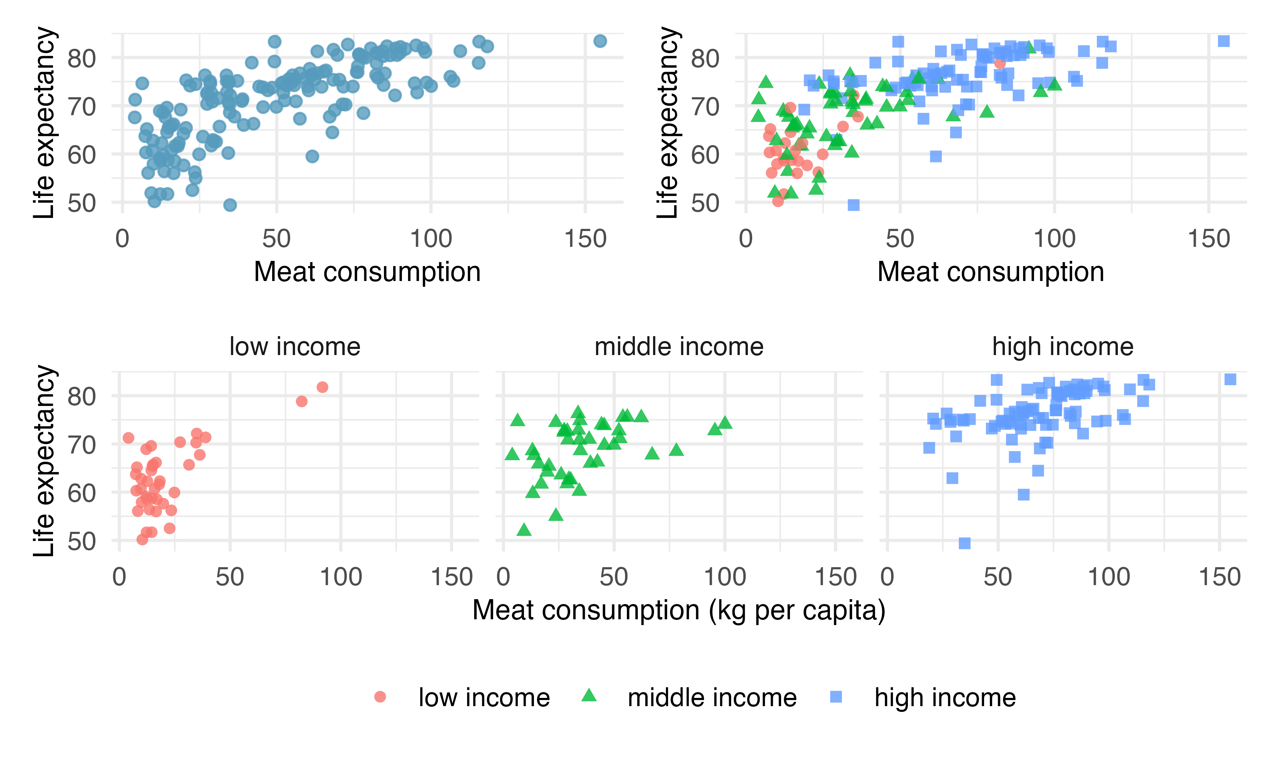
Describe the relationship between meat consumption and life expectancy.
Why do you think the variables are positively associated?
Is the relationship between meat consumption and life expectancy stronger, similar, or weaker when broken down by income bracket in the separate plots along the bottom (as compared with the relationship when combined in the top left figure)?
-
Arrival delays. Consider all of the flights out of New York City in 2013 that flew into Puerto Rico (BQN) or San Francisco (SFO) on the following two airlines: JetBlue (B6) or United Airlines (UA). We consider the relationship between day of the year and arrival delay (in minutes). Note that a negative arrival delay means that the flight arrived early. The figures display a least squares regression line for arrival delay versus time (day of the year).10
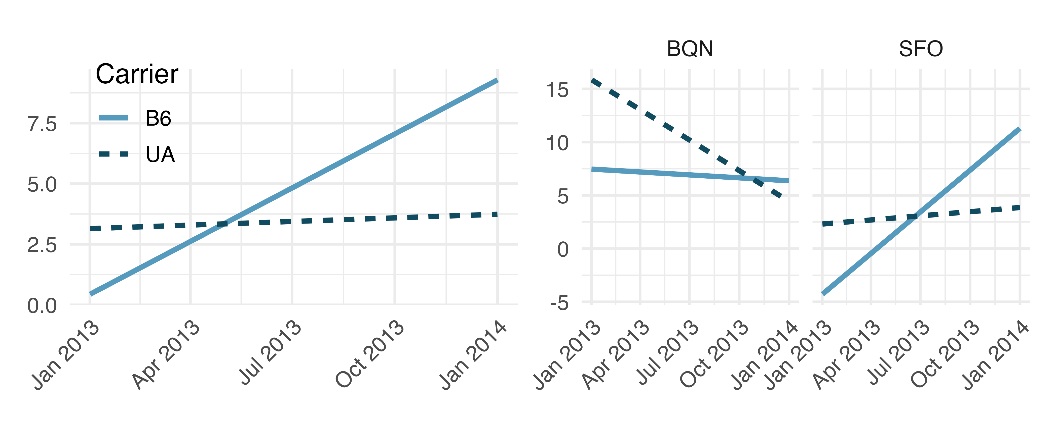
Does it seem like there are differences in arrival delays across time when looking at BQN and SFO airports combined (left figure)? Explain.
Does it seem like there are difference in arrival delays across time when looking at BQN and SFO airports separately (right figure)? Explain.
Would it be more appropriate to display the combined plot or the plots which display the airports separately? Explain.
-
Training for a 5K. Nico signs up for a 5K (a 5,000 metre running race) 30 days prior to the race. They decide to run a 5K every day to train for it, and each day they record the following information:
days_since_start(number of days since starting training),days_till_race(number of days left until the race),mood(poor, good, awesome),tiredness(1-not tired to 10-very tired), andtime(time it takes to run 5K, recorded as mm:ss). Top few rows of the data they collect is shown below. Using these data Nico wants to build a model predictingtimefrom the other variables. Should they include all variables shown above in their model? Why or why not?days_since_start days_till_race mood tiredness time 1 29 good 3 25:45 2 28 poor 5 27:13 3 27 awesome 4 24:13 ... ... ... ... ... -
Multiple regression fact checking. Determine which of the following statements are true and false. For each statement that is false, explain why it is false.
If predictors are collinear, then removing one variable will have no influence on the point estimate of another variable’s coefficient.
Suppose a numerical variable \(x\) has a coefficient of \(b_1 = 2.5\) in the multiple regression model. Suppose also that the first observation has \(x_1 = 7.2\), the second observation has a value of \(x_1 = 8.2\), and these two observations have the same values for all other predictors. Then the predicted value of the second observation will be 2.5 higher than the prediction of the first observation based on the multiple regression model.
If a regression model’s first variable has a coefficient of \(b_1 = 5.7\), then if we are able to influence the data so that an observation will have its \(x_1\) be 1 larger than it would otherwise, the value \(y_1\) for this observation would increase by 5.7.
-
Baby weights and smoking. US Department of Health and Human Services, Centers for Disease Control and Prevention collect information on births recorded in the country. The data used here are a random sample of 1,000 births from 2014. Here, we study the relationship between smoking and weight of the baby. The variable
smokeis coded 1 if the mother is a smoker, and 0 if not. The summary table below shows the results of a linear regression model for predicting the average birth weight of babies, measured in pounds, based on the smoking status of the mother.11 (ICPSR 2014)term estimate std.error statistic p.value (Intercept) 7.270 0.0435 167.22 <0.0001 habitsmoker -0.593 0.1275 -4.65 <0.0001 Write the equation of the regression model.
Interpret the slope in this context, and calculate the predicted birth weight of babies born to smoker and non-smoker mothers.
-
Baby weights and mature moms. The following is a model for predicting baby weight from whether the mom is classified as a
maturemom (35 years or older at the time of pregnancy). (ICPSR 2014)term estimate std.error statistic p.value (Intercept) 7.354 0.103 71.02 <0.0001 matureyounger mom -0.185 0.113 -1.64 0.102 Write the equation of the regression model.
Interpret the slope in this context, and calculate the predicted birth weight of babies born to mature and younger mothers.
-
Movie returns, prediction. A model was fit to predict return-on-investment (ROI) on movies based on release year and genre (Adventure, Action, Drama, Horror, and Comedy). The model output is shown below. (FiveThirtyEight 2015)
term estimate std.error statistic p.value (Intercept) -156.04 169.15 -0.92 0.3565 release_year 0.08 0.08 0.94 0.348 genreAdventure 0.30 0.74 0.40 0.6914 genreComedy 0.57 0.69 0.83 0.4091 genreDrama 0.37 0.62 0.61 0.5438 genreHorror 8.61 0.86 9.97 <0.0001 For a given release year, which genre of movies are predicted, on average, to have the highest predicted return on investment?
The adjusted \(R^2\) of this model is 10.71%. Adding the production budget of the movie to the model increases the adjusted \(R^2\) to 10.84%. Should production budget be added to the model?
-
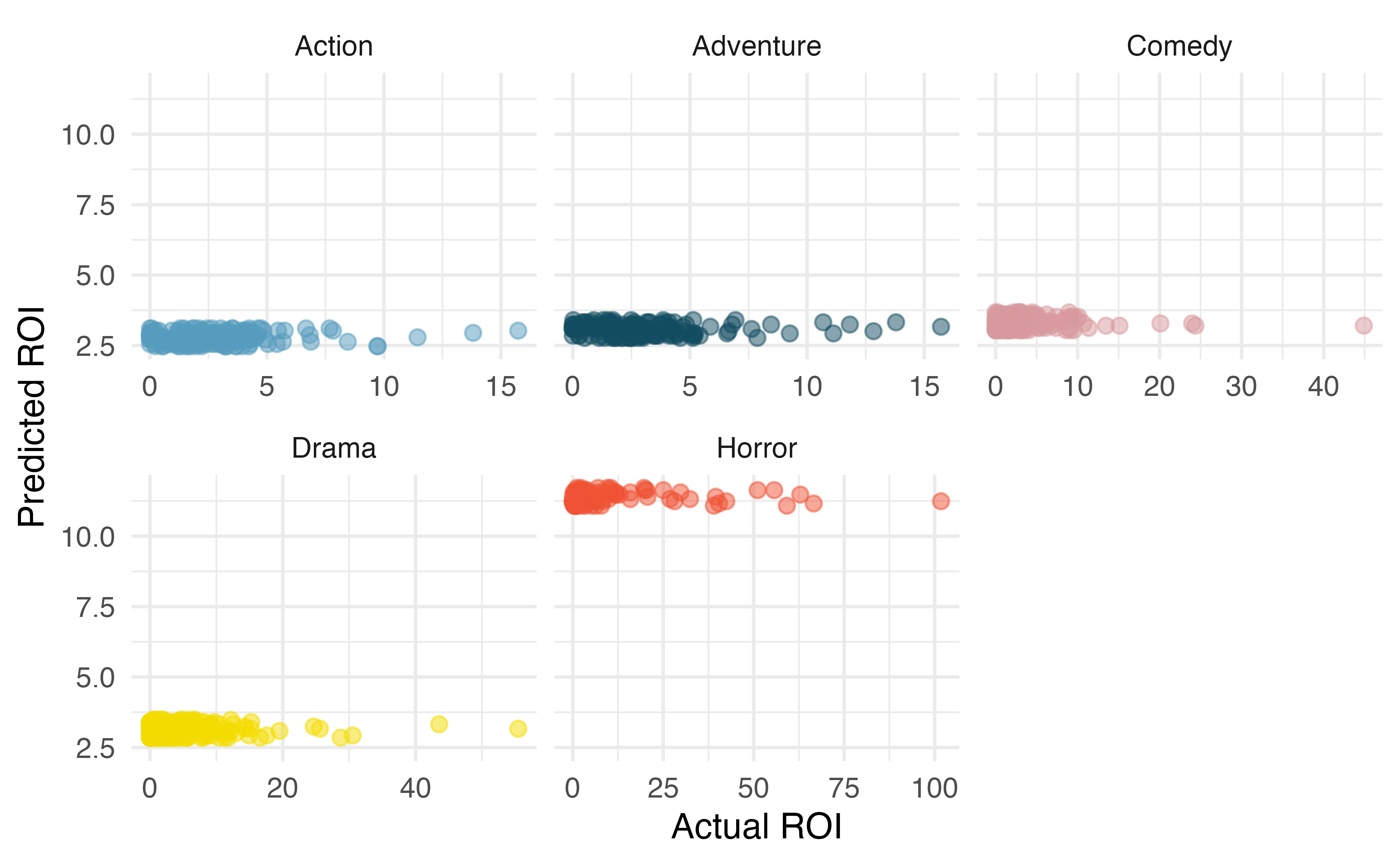
Movie returns by genre. A model was fit to predict return-on-investment (ROI) on movies based on release year and genre (Adventure, Action, Drama, Horror, and Comedy). The plots below show the predicted ROI vs. actual ROI for each of the genres separately. Do these figures support the comment in the FiveThirtyEight.com article that states, “The return-on-investment potential for horror movies is absurd.” Note that the x-axis range varies for each plot. (FiveThirtyEight 2015)
-
Predicting baby weights. A more realistic approach to modeling baby weights is to consider all possibly related variables at once. Other variables of interest include length of pregnancy in weeks (
weeks), mother’s age in years (mage), the sex of the baby (sex), smoking status of the mother (habit), and the number of hospital (visits) visits during pregnancy. Below are three observations from this dataset.weight weeks mage sex visits habit 6.96 37 34 male 14 nonsmoker 8.86 41 31 female 12 nonsmoker 7.51 37 36 female 10 nonsmoker The summary table below shows the results of a regression model for predicting the average birth weight of babies based on all of the variables presented above.
term estimate std.error statistic p.value (Intercept) -3.82 0.57 -6.73 <0.0001 weeks 0.26 0.01 18.93 <0.0001 mage 0.02 0.01 2.53 0.0115 sexmale 0.37 0.07 5.30 <0.0001 visits 0.02 0.01 2.09 0.0373 habitsmoker -0.43 0.13 -3.41 7e-04 Write the equation of the regression model that includes all of the variables.
Interpret the slopes of
weeksandhabitin this context.If we fit a model predicting baby weight from only
habit(whether the mom smokes), we observe a difference in the slope coefficient forhabitin this small model and the slope coefficient forhabitin the larger model. Why might there be a difference?Calculate the residual for the first observation in the dataset.
-
Palmer penguins, predicting body mass. Researchers studying a community of Antarctic penguins collected body measurement (bill length, bill depth, and flipper length measured in millimeters and body mass, measured in grams), species (Adelie, Chinstrap, or Gentoo), and sex (female or male) data on 344 penguins living on three islands (Torgersen, Biscoe, and Dream) in the Palmer Archipelago, Antarctica.12 The summary table below shows the results of a linear regression model for predicting body mass (which is more difficult to measure) from the other variables in the dataset. (Gorman et al. 2014)
term estimate std.error statistic p.value (Intercept) -1461.0 571.3 -2.6 0.011 bill_length_mm 18.2 7.1 2.6 0.0109 bill_depth_mm 67.2 19.7 3.4 7e-04 flipper_length_mm 16.0 2.9 5.5 <0.0001 sexmale 389.9 47.8 8.1 <0.0001 speciesChinstrap -251.5 81.1 -3.1 0.0021 speciesGentoo 1014.6 129.6 7.8 <0.0001 Write the equation of the regression model.
Interpret each one of the slopes in this context.
-
Calculate the residual for a male Adelie penguin that weighs 3,750 grams with the following body measurements:
-
bill_length_mm= 39.1 -
bill_depth_mm= 18.7 -
flipper_length_mm= 181
Does the model overpredict or underpredict this penguin’s weight?
-
The \(R^2\) of this model is 87.5%. Interpret this value in context of the data and the model.
-
Baby weights, backwards elimination. Let’s consider a model that predicts
weightof newborns using several predictors: whether the mother is consideredmature, number ofweeksof gestation, number of hospitalvisitsduring pregnancy, weightgainedby the mother during pregnancy,sexof the baby, and whether the mother smoke cigarettes during pregnancy (habit). (ICPSR 2014)The adjusted \(R^2\) of the full model is 0.326. We remove each variable one by one, refit the model, and record the adjusted \(R^2\). Which, if any, variable should be removed from the model?
- Drop
mature: 0.321 - Drop
weeks: 0.061 - Drop
visits: 0.326 - Drop
gained: 0.327 - Drop
sex: 0.301
- Drop
-
Palmer penguins, backwards elimination. The following full model is built to predict the weights of three species (Adelie, Chinstrap, or Gentoo) of penguins living in the Palmer Archipelago, Antarctica. (Gorman et al. 2014)
term estimate std.error statistic p.value (Intercept) -1461.0 571.3 -2.6 0.011 bill_length_mm 18.2 7.1 2.6 0.0109 bill_depth_mm 67.2 19.7 3.4 7e-04 flipper_length_mm 16.0 2.9 5.5 <0.0001 sexmale 389.9 47.8 8.1 <0.0001 speciesChinstrap -251.5 81.1 -3.1 0.0021 speciesGentoo 1014.6 129.6 7.8 <0.0001 The adjusted \(R^2\) of the full model is 0.9. In order to evaluate whether any of the predictors can be dropped from the model without losing predictive performance of the model, the researchers dropped one variable at a time, refit the model, and recorded the adjusted \(R^2\) of the smaller model. These values are given below.
- Drop
bill_length_mm: 0.87 - Drop
bill_depth_mm: 0.869 - Drop
flipper_length_mm: 0.861 - Drop
sex: 0.845 - Drop
species: 0.821
Which, if any, variable should be removed from the model first?
- Drop
-
Baby weights, forward selection. Using information on the mother and the sex of the baby (which can be determined prior to birth), we want to build a model that predicts the birth weight of babies. In order to do so, we will evaluate six candidate predictors: whether the mother is considered
mature, number ofweeksof gestation, number of hospitalvisitsduring pregnancy, weightgainedby the mother during pregnancy,sexof the baby, and whether the mother smoke cigarettes during pregnancy (habit). And we will make a decision about including them in the model using forward selection and adjusted \(R^2\). Below are the six models we evaluate and their adjusted \(R^2\) values. (ICPSR 2014)- Predict
weightfrommature: 0.002 - Predict
weightfromweeks: 0.3 - Predict
weightfromvisits: 0.034 - Predict
weightfromgained: 0.021 - Predict
weightfromsex: 0.018 - Predict
weightfromhabit: 0.021
Which variable should be added to the model first?
- Predict
-
Palmer penguins, forward selection. Using body measurement and other relevant data on three species (Adelie, Chinstrap, or Gentoo) of penguins living in the Palmer Archipelago, Antarctica, we want to predict their body mass. In order to do so, we will evaluate five candidate predictors and make a decision about including them in the model using forward selection and adjusted \(R^2\). Below are the five models we evaluate and their adjusted \(R^2\) values:
- Predict body mass from
bill_length_mm: 0.352 - Predict body mass from
bill_depth_mm: 0.22 - Predict body mass from
flipper_length_mm: 0.758 - Predict body mass from
sex: 0.178 - Predict body mass from
species: 0.668
Which variable should be added to the model first?
- Predict body mass from
When
verified_incometakes a value ofVerified, then the corresponding variable takes a value of 1 while the other is 0: \(11.10 + 1.42 \times 0 + 3.25 \times 1 = 14.35.\) The average interest rate for these borrowers is 14.35%.↩︎Each of the coefficients gives the incremental interest rate for the corresponding level relative to the
Not Verifiedlevel, which is the reference level. For example, for a borrower whose income source and amount have been verified, the model predicts that they will have a 3.25% higher interest rate than a borrower who has not had their income source or amount verified.↩︎Relative to the
Not Verifiedcategory, theVerifiedcategory has an interest rate of 3.25% higher, while theSource Verifiedcategory is only 1.42% higher. Thus,Verifiedborrowers will tend to get an interest rate about \(3.25\% - 1.42\% = 1.83\%\) higher thanSource Verifiedborrowers.↩︎All else held constant, for each additional inquiry into the applicant’s credit during the last 12 months, we would expect the interest rate for the loan to be higher, on average, by 0.23 points.↩︎
To compute the residual, we first need the predicted value, which we compute by plugging values into the equation from earlier. For example, \(\texttt{verified\_income}_{\texttt{Source Verified}}\) takes a value of 0, \(\texttt{verified\_income}_{\texttt{Verified}}\) takes a value of 1 (since the borrower’s income source and amount were verified), \(\texttt{debt\_to\_income}\) was 18.01, and so on. This leads to a prediction of \(\widehat{\texttt{interest\_rate}}_1 = 17.84\). The observed interest rate was 14.07%, which leads to a residual of \(e_1 = 14.07 - 17.84 = -3.77\).↩︎
Many of the variables do take a value 0 for at least one data point, and for those variables, it is reasonable. However, one variable never takes a value of zero:
term, which describes the length of the loan, in months. Iftermis set to zero, then the loan must be paid back immediately; the borrower must give the money back as soon as they receive it, which means it is not a real loan. Ultimately, the interpretation of the intercept in this setting is not insightful.↩︎\(R^2 = 1 - \frac{18.53}{25.01} = 0.2591\).↩︎
\(R_{adj}^2 = 1 - \frac{18.53}{25.01}\times \frac{10000-1}{10000-9-1} = 0.2584\). While the difference is very small, it will be important when we fine tune the model in the next section.↩︎
The unadjusted \(R^2\) would stay the same and the adjusted \(R^2\) would go down.↩︎
The
flightsdata used in this exercise can be found in the nycflights13 R package.↩︎The
births14data used in this exercise can be found in the openintro R package.↩︎The
penguinsdata used in this exercise can be found in the palmerpenguins R package.↩︎