10 Applications: Model
10.1 Case study: Houses for sale
Take a walk around your neighborhood and you’ll probably see a few houses for sale, and you might be able to look up its price online. You’ll note that house prices are somewhat arbitrary – the homeowners get to decide the listing price, and many criteria factor into this decision, e.g., what do comparable houses (“comps” in real estate speak) sell for, how quickly they need to sell the house, etc.
In this case study we’ll formalize the process of determining the listing price of a house by using data on current home sales. In November of 2020, information on 98 houses in the Duke Forest neighborhood of Durham, NC were scraped from Zillow. The homes were all recently sold at the time of data collection, and the goal of the project was to build a model for predicting the sale price based on a particular home’s characteristics. The first four homes are shown in Table 10.1, and descriptions of each variable are shown in Table 10.2.
The duke_forest data can be found in the openintro R package.
duke_forest.
| price | bed | bath | area | year_built | cooling | lot |
|---|---|---|---|---|---|---|
| 1,520,000 | 3 | 4 | 6,040 | 1,972 | central | 0.97 |
| 1,030,000 | 5 | 4 | 4,475 | 1,969 | central | 1.38 |
| 420,000 | 2 | 3 | 1,745 | 1,959 | central | 0.51 |
| 680,000 | 4 | 3 | 2,091 | 1,961 | central | 0.84 |
duke_forest dataset.
| Variable | Description |
|---|---|
| price | Sale price, in USD |
| bed | Number of bedrooms |
| bath | Number of bathrooms |
| area | Area of home, in square feet |
| year_built | Year the home was built |
| cooling | Cooling system: central or other (other is baseline) |
| lot | Area of the entire property, in acres |
10.1.1 Correlating with price
As mentioned, the goal of the data collection was to build a model for the sale price of homes. While using multiple predictor variables is likely preferable to using only one variable, we start by learning about the variables themselves and their relationship to price. Figure 10.1 shows scatterplots describing price as a function of each of the predictor variables. All of the variables seem to be positively associated with price (higher values of the variable are matched with higher price values).
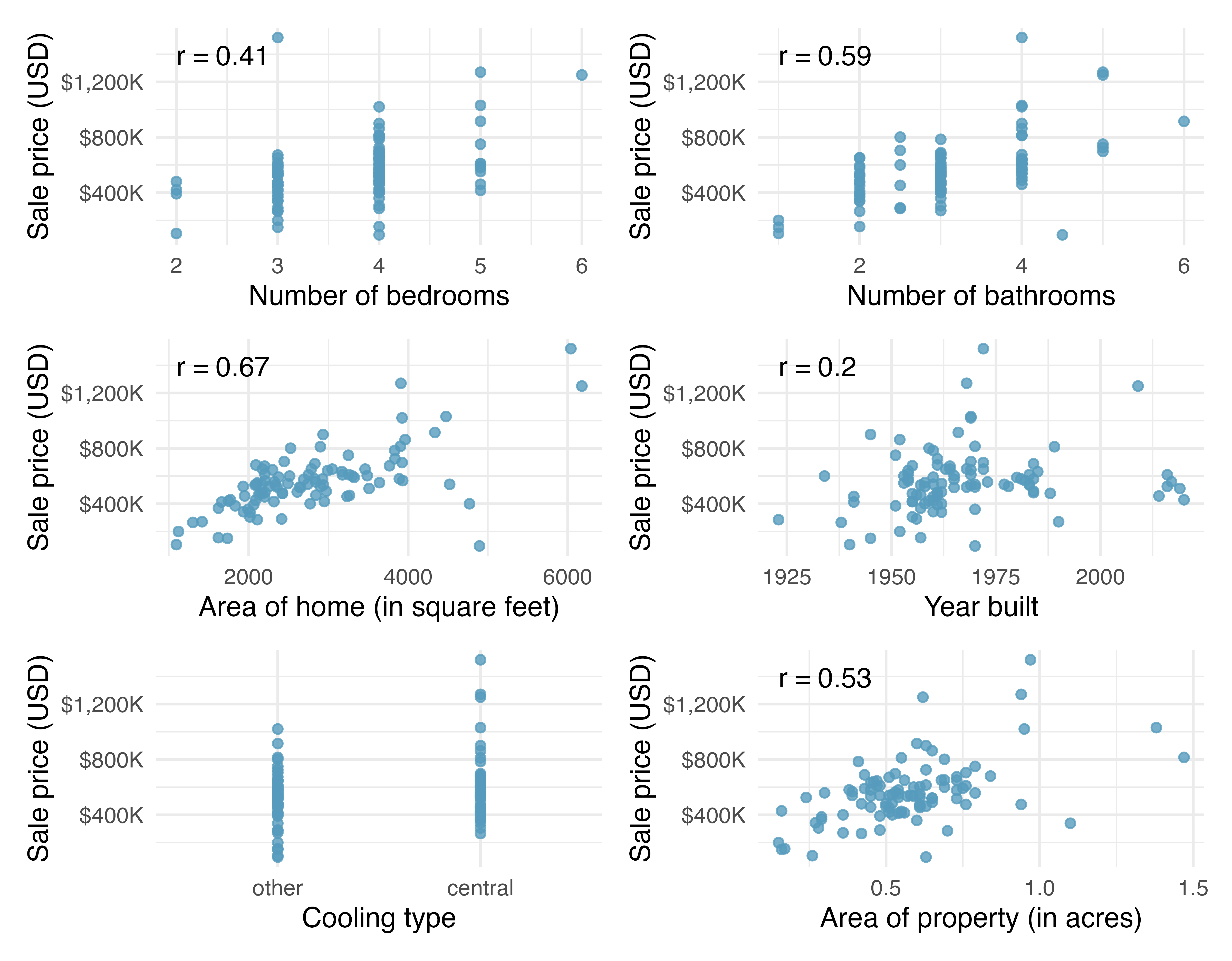
In Figure 10.1 there does not appear to be a correlation value calculated for the predictor variable, cooling. Why not? Can the variable still be used in the linear model?1
In Figure 10.1 which variable seems to be most informative for predicting house price? Provide two reasons for your answer.
The area of the home is the variable which is most highly correlated with price. Additionally, the scatterplot for price vs. area seems to show a strong linear relationship between the two variables. Note that the correlation coefficient and the scatterplot linearity will often give the same conclusion. However, recall that the correlation coefficient is very sensitive to outliers, so it is always wise to look at the scatterplot even when the variables are highly correlated.
10.1.2 Modeling price with area
A linear model was fit to predict price from area. The resulting model information is given in Table 10.3.
| term | estimate | std.error | statistic | p.value |
|---|---|---|---|---|
| (Intercept) | 116,652 | 53,302 | 2.19 | 0.0311 |
| area | 159 | 18 | 8.78 | <0.0001 |
| Adjusted R-sq = 0.4394 | ||||
| df = 96 | ||||
Interpret the value of \(b_1\) = 159 in the context of the problem.2
Using the output in Table 10.3, write out the model for predicting price from area.3
The residuals from the linear model can be used to assess whether a linear model is appropriate. Figure 10.2 plots the residuals \(e_i = y_i - \hat{y}_i\) on the \(y\)-axis and the fitted (or predicted) values \(\hat{y}_i\) on the \(x\)-axis.
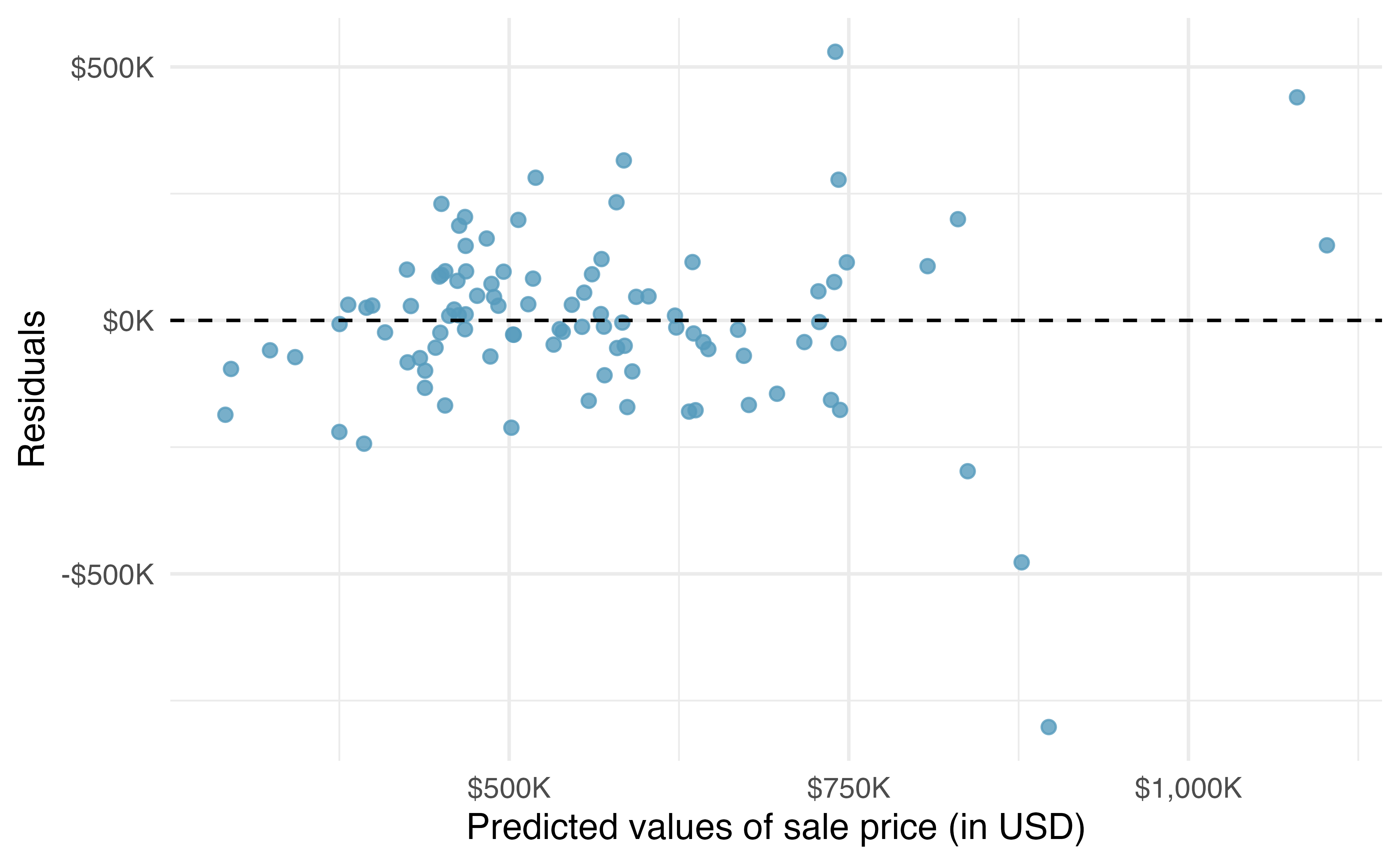
What aspect(s) of the residual plot indicate that a linear model is appropriate? What aspect(s) of the residual plot seem concerning when fitting a linear model?4
10.1.3 Modeling price with multiple variables
It seems as though the predictions of home price might be more accurate if more than one predictor variable was used in the linear model. Table 10.4 displays the output from a linear model of price regressed on area, bed, bath, year_built, cooling, and lot.
| term | estimate | std.error | statistic | p.value |
|---|---|---|---|---|
| (Intercept) | -2,910,715 | 1,787,934 | -1.63 | 0.107 |
| area | 102 | 23 | 4.42 | <0.0001 |
| bed | -13,692 | 25,928 | -0.53 | 0.5987 |
| bath | 41,076 | 24,662 | 1.67 | 0.0993 |
| year_built | 1,459 | 914 | 1.60 | 0.1139 |
| coolingcentral | 84,065 | 30,338 | 2.77 | 0.0068 |
| lot | 356,141 | 75,940 | 4.69 | <0.0001 |
| Adjusted R-sq = 0.5896 | ||||
| df = 90 | ||||
Using Table 10.4, write out the linear model of price on the six predictor variables.
\[ \begin{aligned} \widehat{\texttt{price}} = -2,910,715 &+ 102 \times \texttt{area} \\ &- 13,692 \times \texttt{bed} \\ &+ 41,076 \times \texttt{bath} \\ &+ 1,459 \times \texttt{year\_built} \\ &+ 84,065 \times \texttt{cooling}_{\texttt{central}} \\ &+ 356,141 \times \texttt{lot} \end{aligned} \]
The value of the estimated coefficient on \(\texttt{cooling}_{\texttt{central}}\) is \(b_5 = 84,065.\) Interpret the value of \(b_5\) in the context of the problem.5
A friend suggests that maybe you do not need all six variables to have a good model for price. You consider taking a variable out, but you aren’t sure which one to remove.
Results corresponding to the full model for the housing data are shown in Table 10.4. How should we proceed under the backward elimination strategy?
Our baseline adjusted \(R^2\) from the full model is 0.59, and we need to determine whether dropping a predictor will improve the adjusted \(R^2\). To check, we fit models that each drop a different predictor, and we record the adjusted \(R^2\):
- Excluding
area: 0.506 - Excluding
bed: 0.593 - Excluding
bath: 0.582 - Excluding
year_built: 0.583 - Excluding
cooling: 0.559 - Excluding
lot: 0.489
The model without bed has the highest adjusted \(R^2\) of 0.593, higher than the adjusted \(R^2\) for the full model. Because eliminating bed leads to a model with a higher adjusted \(R^2\) than the full model, we drop bed from the model. It might seem counter-intuitive to exclude number of bedrooms from the model. After all, we would expect homes with more bedrooms to cost more, and we can see a clear relationship between number of bedrooms and sale price in Figure 10.1. However, note that area is still in the model, and it’s quite likely that the area of the home and the number of bedrooms are highly associated. Therefore, the model already has information on “how much space is available in the house” with the inclusion of area.
Since we eliminated a predictor from the model in the first step, we see whether we should eliminate any additional predictors. Our baseline adjusted \(R^2\) is now 0.593. We fit another set of new models, which consider eliminating each of the remaining predictors in addition to bed:
- Excluding
bedandarea: 0.51 - Excluding
bedandbath: 0.586 - Excluding
bedandyear_built: 0.586 - Excluding
bedandcooling: 0.563 - Excluding
bedandlot: 0.493
None of these models lead to an improvement in adjusted \(R^2\), so we do not eliminate any of the remaining predictors.
That is, after backward elimination, we are left with the model that keeps all predictors except bed, which we can summarize using the coefficients from Table 10.5.
| term | estimate | std.error | statistic | p.value |
|---|---|---|---|---|
| (Intercept) | -2,952,641 | 1,779,079 | -1.66 | 0.1004 |
| area | 99 | 22 | 4.44 | <0.0001 |
| bath | 36,228 | 22,799 | 1.59 | 0.1155 |
| year_built | 1,466 | 910 | 1.61 | 0.1107 |
| coolingcentral | 83,856 | 30,215 | 2.78 | 0.0067 |
| lot | 357,119 | 75,617 | 4.72 | <0.0001 |
| Adjusted R-sq = 0.5929 | ||||
| df = 91 | ||||
Then, the linear model for predicting sale price based on this model is as follows:
\[ \begin{aligned} \widehat{\texttt{price}} = &-2,952,641 + 99 \times \texttt{area} + 36,228 \times \texttt{bath} + 1,466 \times \texttt{year\_built} \\ &+ 83,856 \times \texttt{cooling}_{\texttt{central}} + 357,119 \times \texttt{lot} \end{aligned} \]
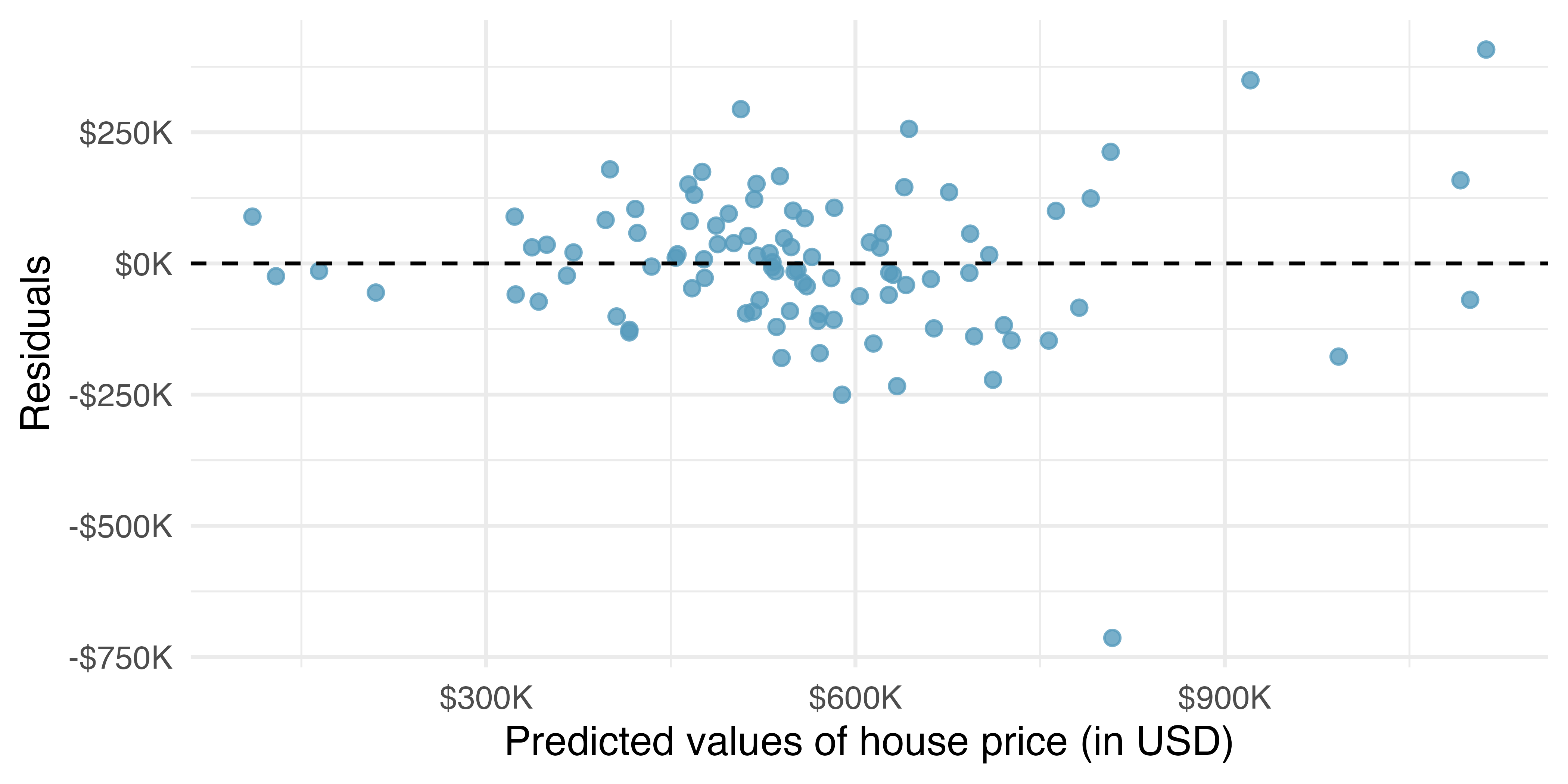
The residual plot for the model with all of the predictor variables except bed is given in Figure 10.3. How do the residuals in Figure 10.3 compare to the residuals in Figure 10.2?
The residuals, for the most part, are randomly scattered around 0. However, there is one extreme outlier with a residual of -$750,000, a house whose actual sale price is a lot lower than its predicted price. Also, we observe again that the residuals are quite large for expensive homes.
Consider a house with 1,803 square feet, 2.5 bathrooms, 0.145 acres, built in 1941, that has central air conditioning. What is the predicted price of the home?6
If you later learned that the house (with a predicted price of $297,570) had recently sold for $804,133, would you think the model was terrible? What if you learned that the house was in California?7
10.2 Interactive R tutorials
Navigate the concepts you’ve learned in this part in R using the following self-paced tutorials. All you need is your browser to get started!
You can also access the full list of tutorials supporting this book here.
10.3 R labs
Further apply the concepts you’ve learned in this part in R with computational labs that walk you through a data analysis case study.
You can also access the full list of labs supporting this book here.
The correlation coefficient can only be calculated to describe the relationship between two numerical variables. The predictor variable
coolingis categorical, not numerical. It can, however, be used in the linear model as a binary indicator variable coded, for example, with a1for central and0for other.↩︎For each additional square foot of house, we would expect such houses to cost, on average, $159 more.↩︎
\(\widehat{\texttt{price}} = 116,652 + 159 \times \texttt{area}\)↩︎
The residual plot shows that the relationship between
areaandpriceof a home is indeed linear. However, the residuals are quite large for expensive homes. The large residuals indicate potential outliers or increasing variability, either of which could warrant more involved modeling techniques than are presented in this chapter.↩︎The coefficient indicates that if all the other variables are kept constant, homes with central air conditioning cost $84,065 more, on average.↩︎
\(\widehat{\texttt{price}} = -2,952,641 + 99 \times 1803 + 36,228 \times 2.5 + 1,466 \times 1941 + 83,856 \times 1 + 357,119 \times 0.145 = \$297,570.\)↩︎
A residual of $506,563 is reasonably big. Note that the large residuals (except a few homes) in Figure 10.3 are closer to $250,000 (about half as big). After we learn that the house is in California, we realize that the model shouldn’t be applied to the new home at all! The original data are from Durham, NC, and models based on the Durham, NC data should be used only to explore patterns in prices for homes in Durham, NC.↩︎