17 Inference for comparing two proportions
We now extend the methods from Chapter 16 to apply confidence intervals and hypothesis tests to differences in population proportions that come from two groups, Group 1 and Group 2: \(p_1 - p_2.\)
In our investigations, we’ll identify a reasonable point estimate of \(p_1 - p_2\) based on the sample, and you may have already guessed its form: \(\hat{p}_1 - \hat{p}_2.\) Then we’ll look at the inferential analysis in three different ways: using a randomization test, applying bootstrapping for interval estimates, and, if we verify that the point estimate can be modeled using a normal distribution, we compute the estimate’s standard error, and we apply the mathematical framework.
17.1 Randomization test for the difference in proportions
17.1.1 Observed data
Let’s take another look at the cardiopulmonary resuscitation (CPR) study we introduced in Section 14.2. The experiment consisted of two treatments on patients who underwent CPR for a heart attack and were subsequently admitted to a hospital. Each patient was randomly assigned to either receive a blood thinner (treatment group) or not receive a blood thinner (control group). The outcome variable of interest was whether the patient survived for at least 24 hours. (Böttiger et al. 2001)
The results are summarized in Table 17.1 (which is a replica of Table 14.2). 11 out of the 50 patients in the control group and 14 out of the 40 patients in the treatment group survived.
| Group | Died | Survived | Total |
|---|---|---|---|
| Control | 39 | 11 | 50 |
| Treatment | 26 | 14 | 40 |
| Total | 65 | 25 | 90 |
Is this an observational study or an experiment? What implications does the study type have on what can be inferred from the results?1
In this study, a larger proportion of patients who received blood thinner after CPR,\(\hat{p}_T = \frac{14}{40} = 0.35,\) survived compared to those who did not receive blood thinner, \(\hat{p}_C = \frac{11}{50} = 0.22.\) However, based on these observed proportions alone, we cannot determine whether the difference (\(\hat{p}_T - \hat{p}_C = 0.35 - 0.22 = 0.13\)) provides convincing evidence that blood thinner usage after CPR is effective.
As we saw in Chapter 11, we can re-randomize the responses (survived or died) to the treatment conditions assuming the null hypothesis is true and compute possible differences in proportions. The process by which we randomize observations to two groups is summarized and visualized in Figure 11.8).
17.1.2 Variability of the statistic
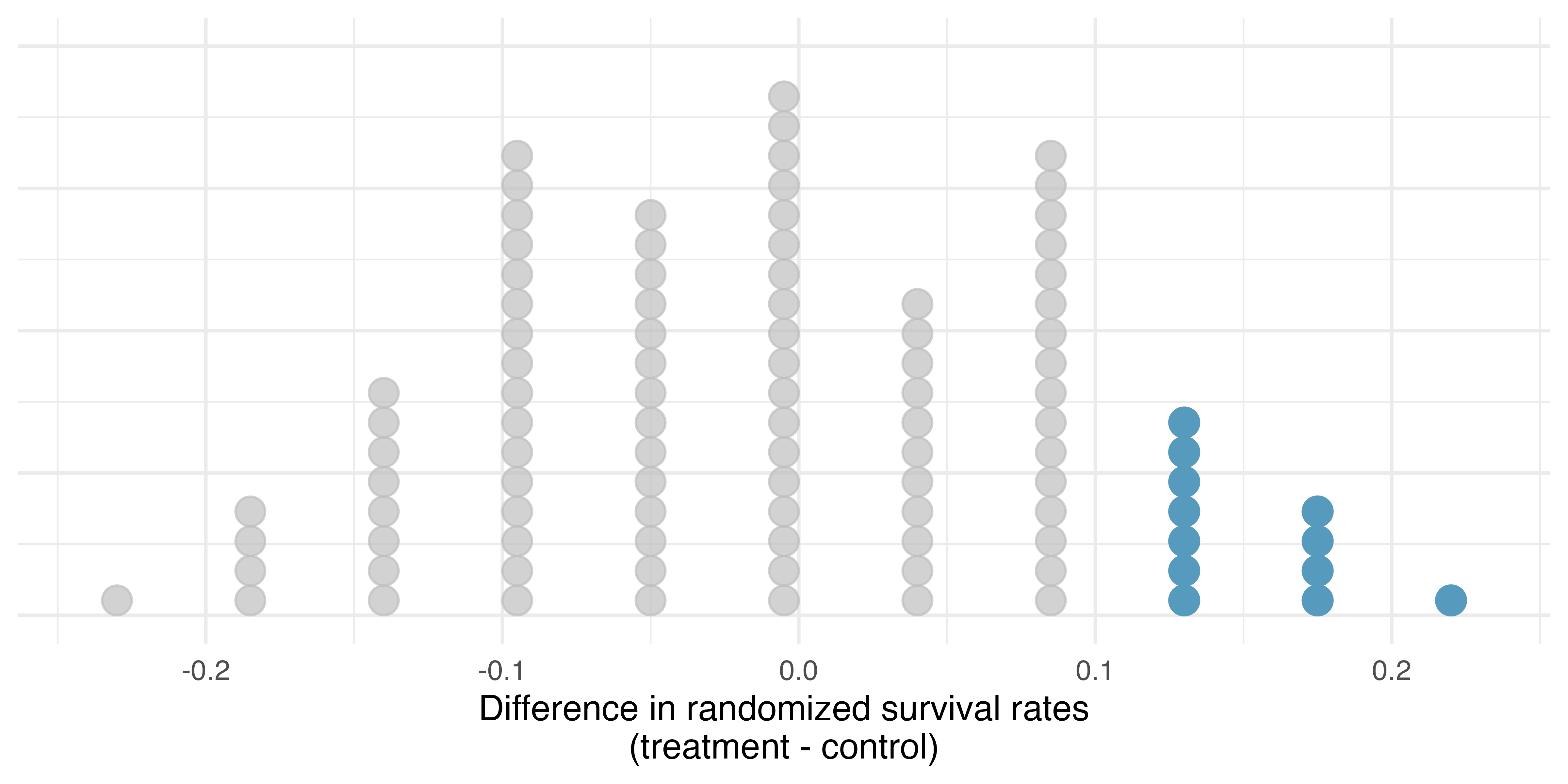
Figure 17.1 shows a stacked plot of the differences found from 100 randomization simulations (i.e., repeated iterations as described in Figure 11.8, where each dot represents a simulated difference between the infection rates (control rate minus treatment rate).
17.1.3 Observed statistic vs null statistics
Note that the distribution of these simulated differences is centered around 0. We simulated the differences assuming that the independence model was true, that blood thinners after CPR have no effect on survival. Under the null hypothesis, we expect the difference to be near zero with some random fluctuation, where near is pretty generous in this case since the sample sizes are so small in this study.
How often would you observe a difference of at least 13% (0.13) according to Figure 17.1? Is this a rare event?
It appears that a difference of at least 13% due to chance alone, if the null hypothesis was true would happen about 12% of the time according to Figure 17.1. This is not a very rare event.
The difference of 13% not being a rare event suggests two possible interpretations of the results of the study:
- \(H_0\) Independence model. Blood thinners after CPR have no effect on survival, and we just happened to observe a difference that would only occur on a rare occasion.
- \(H_A\) Alternative model. Blood thinners after CPR increase chance of survival, and the difference we observed was actually due to the blood thinners after CPR being effective at increasing the chance of survival, which explains the difference of 13%.
Since we determined that the outcome is not that rare (12% chance of observing a difference of 13% or more under the assumption that blood thinners after CPR have no effect on survival), we fail to reject \(H_0\), and conclude that the study results do not provide strong evidence against the independence model. This does not mean that we have proved that blood thinners are not effective, it just means that this study does not provide convincing evidence that they are effective in this setting.
Statistical inference, is built on evaluating how likely such differences are to occur due to chance if in fact the null hypothesis is true. In statistical inference, data scientists evaluate which model is most reasonable given the data. Errors do occur, just like rare events, and we might choose the wrong model. While we do not always choose correctly, statistical inference gives us tools to control and evaluate how often these errors occur.
17.2 Bootstrap confidence interval for the difference in proportions
In Section 17.1, we worked with the randomization distribution to understand the distribution of \(\hat{p}_1 - \hat{p}_2\) when the null hypothesis \(H_0: p_1 - p_2 = 0\) is true. Now, through bootstrapping, we study the variability of \(\hat{p}_1 - \hat{p}_2\) without assuming the null hypothesis is true.
17.2.1 Observed data
Reconsider the CPR data from Section 17.1 which is provided in Table 14.2. Again, we use the difference in sample proportions as the observed statistic of interest. Here, the value of the statistic is: \(\hat{p}_T - \hat{p}_C = 0.35 - 0.22 = 0.13.\)
17.2.2 Variability of the difference in sample proportions
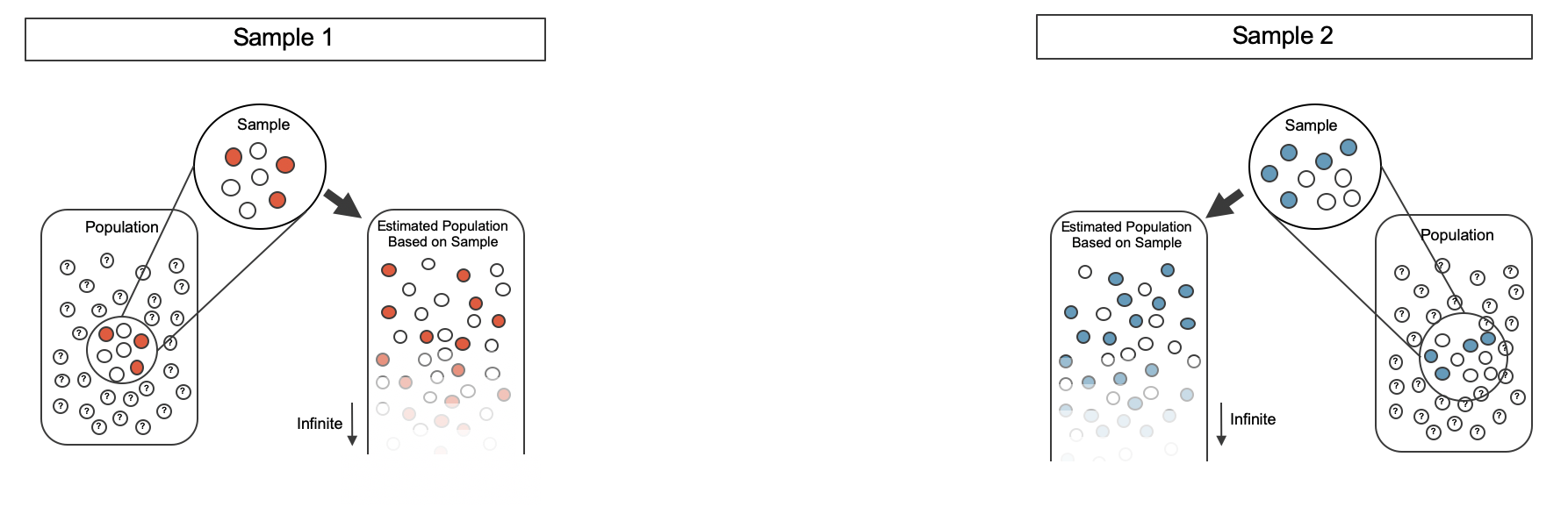
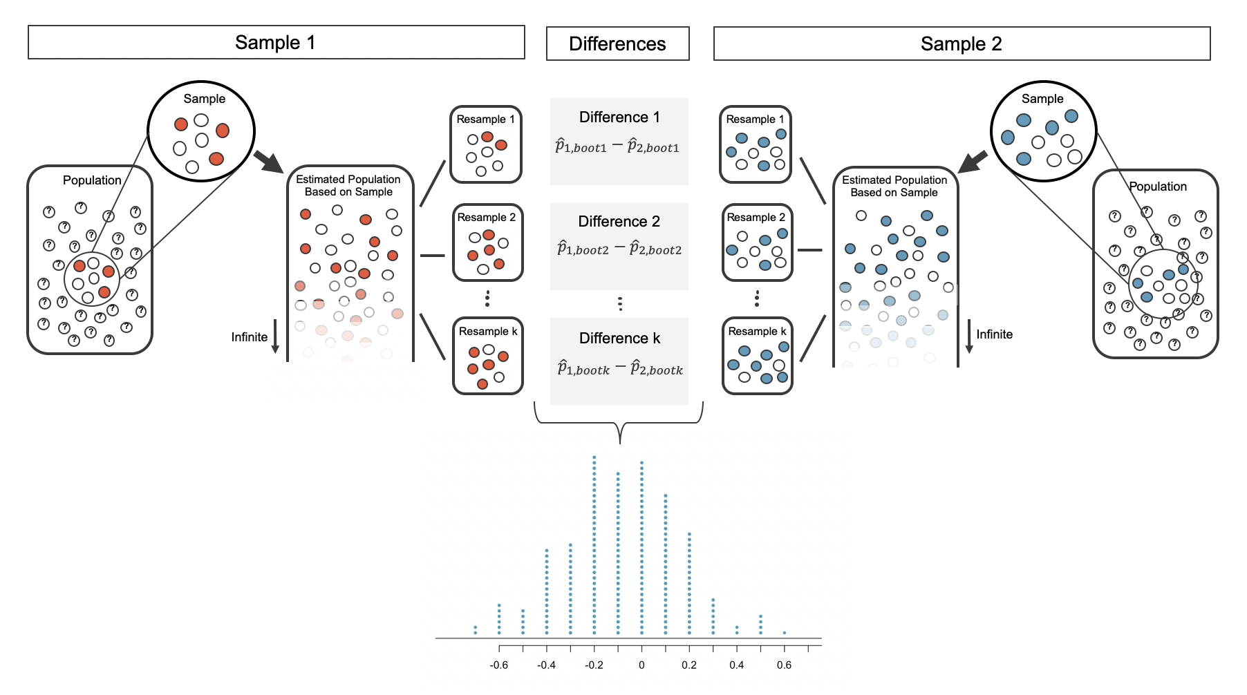
The bootstrap method applied to two samples is an extension of the method described in Chapter 12. Now, we have two samples, so each sample estimates the population from which they came. In the CPR setting, the treatment sample estimates the population of all individuals who have gotten (or will get) the treatment; the control sample estimates the population of all individuals who do not get the treatment and are controls. Figure 17.2 extends Figure 12.1 to show the bootstrapping process from two samples simultaneously.
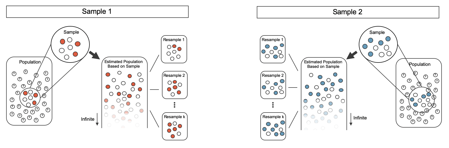
As before, once the population is estimated, we can randomly resample observations to create bootstrap samples, as seen in Figure 17.3.
The variability of the statistic (the difference in sample proportions) can be calculated by taking one bootstrap resample from Sample 1 and one bootstrap resample from Sample 2 and calculating the difference in the bootstrap proportions.
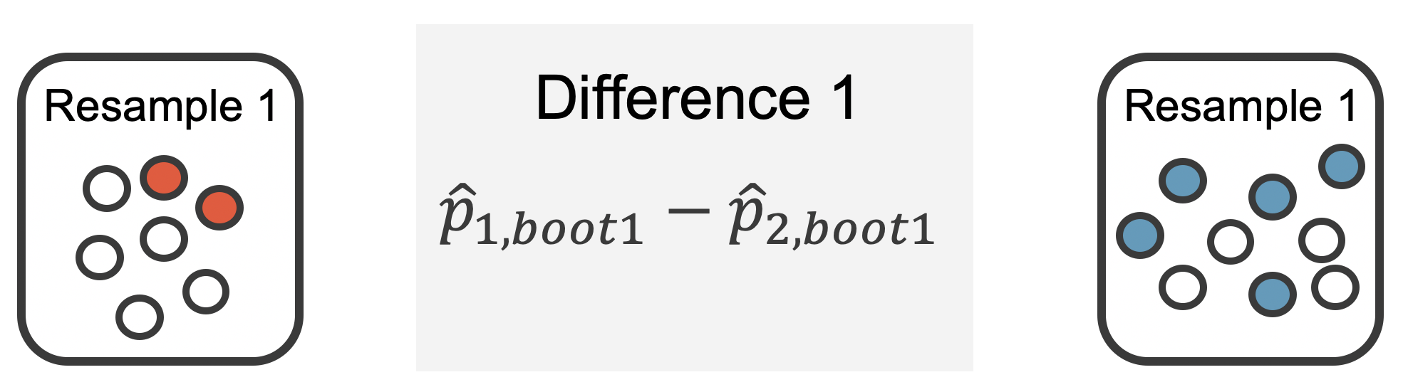
As always, the variability of the difference in proportions can only be estimated by repeated simulations, in this case, repeated bootstrap resamples. Figure 17.4 shows multiple bootstrap differences calculated for each of the repeated bootstrap samples.
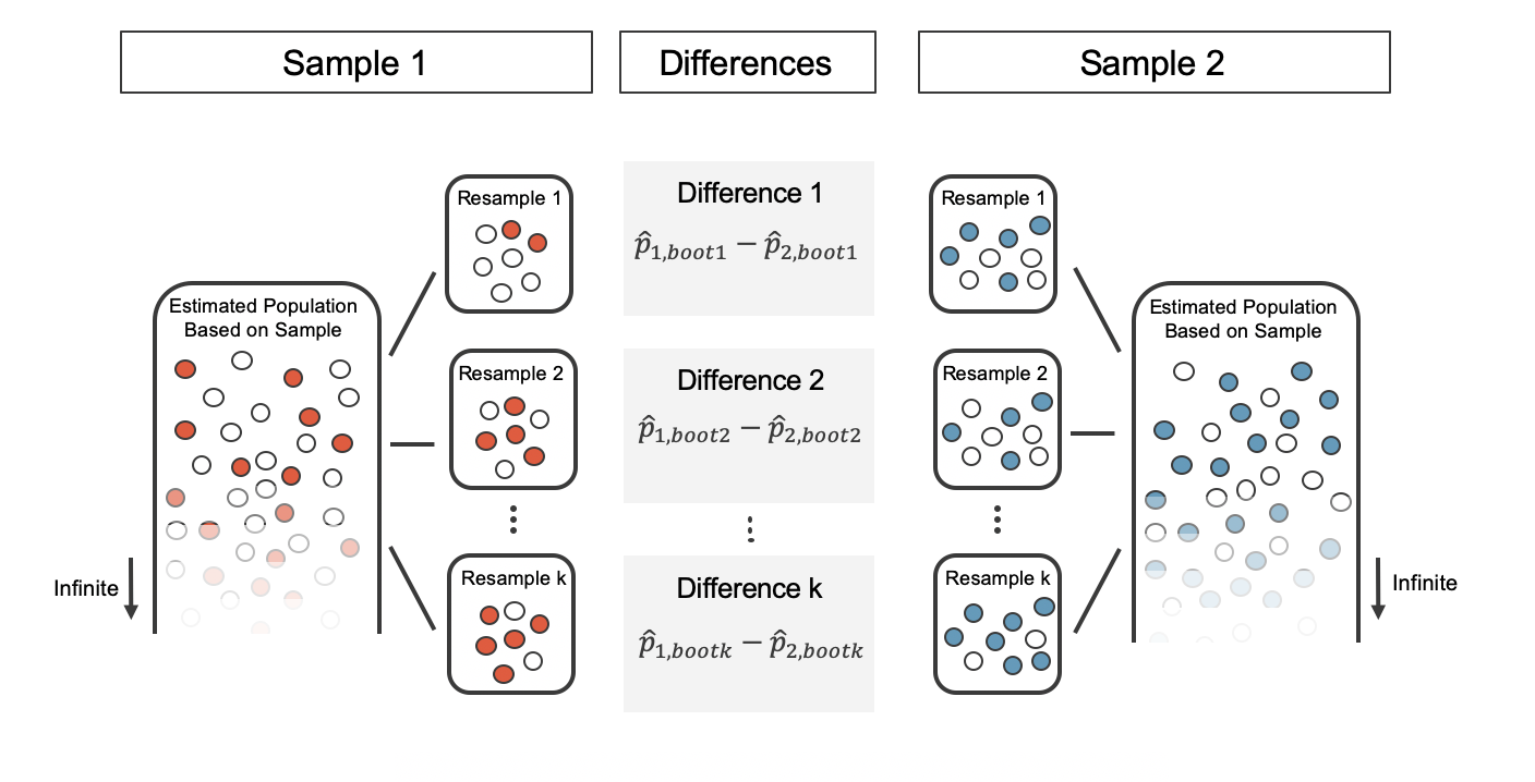
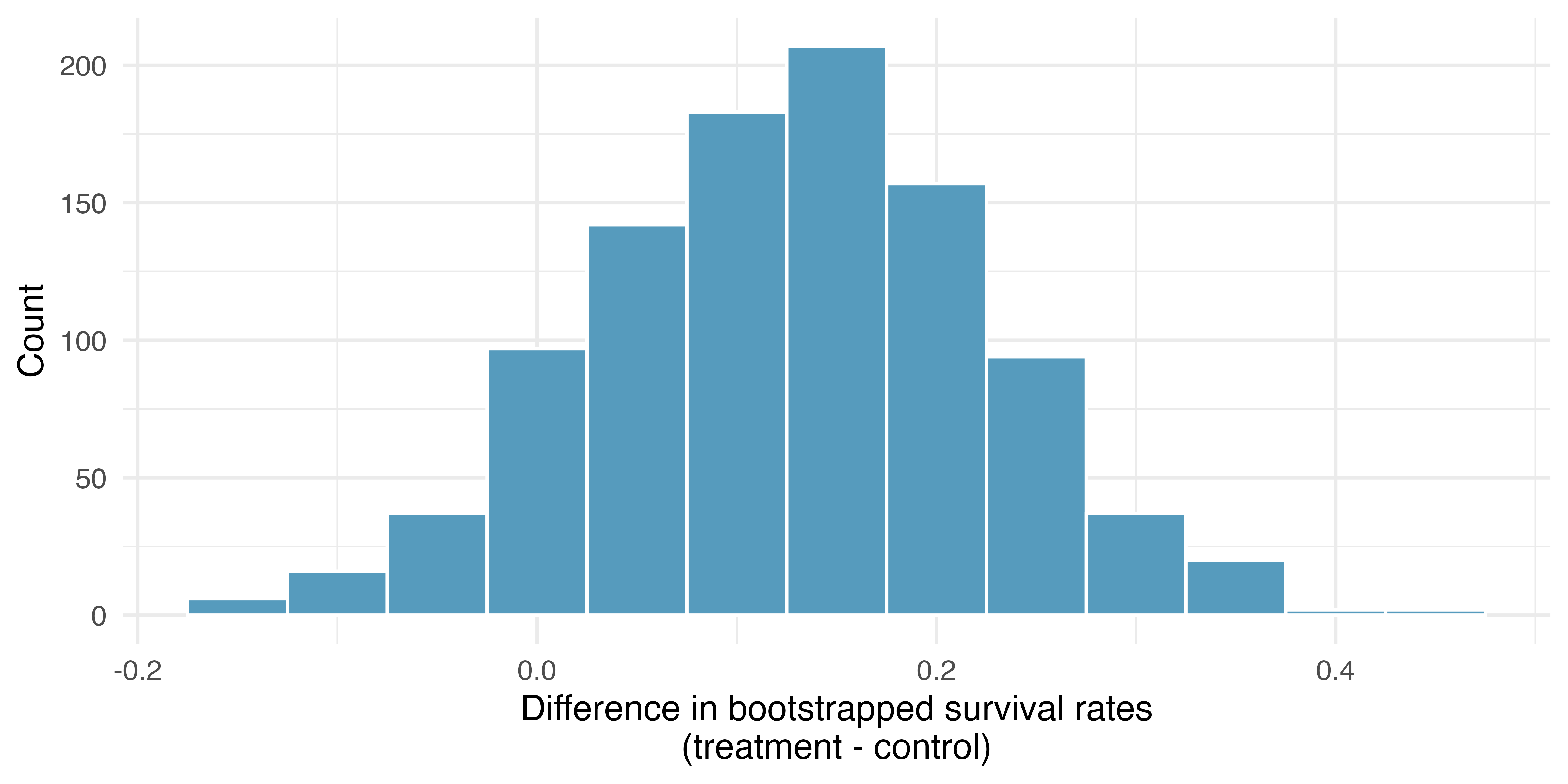
Repeated bootstrap simulations lead to a bootstrap sampling distribution of the statistic of interest, here the difference in sample proportions. Figure 17.6 visualizes the process and Figure 17.7 shows 1,000 bootstrap differences in proportions for the CPR data. Note that the CPR data includes 40 and 50 people in the respective groups, and the illustrated example includes 7 and 9 people in the two groups. Accordingly, the variability in the distribution of sample proportions is higher for the illustrated example. As you will see in the mathematical models discussed in Section 17.3, large sample sizes lead to smaller standard errors for a difference in proportions.
17.2.3 Bootstrap percentile vs. SE confidence intervals
Figure 17.7 provides an estimate for the variability of the difference in survival proportions from sample to sample. The values in the histogram can be used in two different ways to create a confidence interval for the parameter of interest: \(p_1 - p_2\).
As in Chapter 12, the bootstrap confidence interval can be calculated directly from the bootstrapped differences in Figure 17.7. The interval created from the percentiles of the distribution is called the percentile interval. Note that here we calculate the 90% confidence interval by finding the \(5^{th}\) and \(95^{th}\) percentile values from the bootstrapped differences. The bootstrap 5 percentile proportion is -0.032 and the 95 percentile is 0.284. The result is: we are 90% confident that, in the population, the true difference in probability of survival for individuals receiving blood thinners after CPR is between -0.032 lower and 0.284 higher than those who did not receive blood thinners. The interval shows that we do not have much definitive evidence of the effect of blood thinners, one way or another.
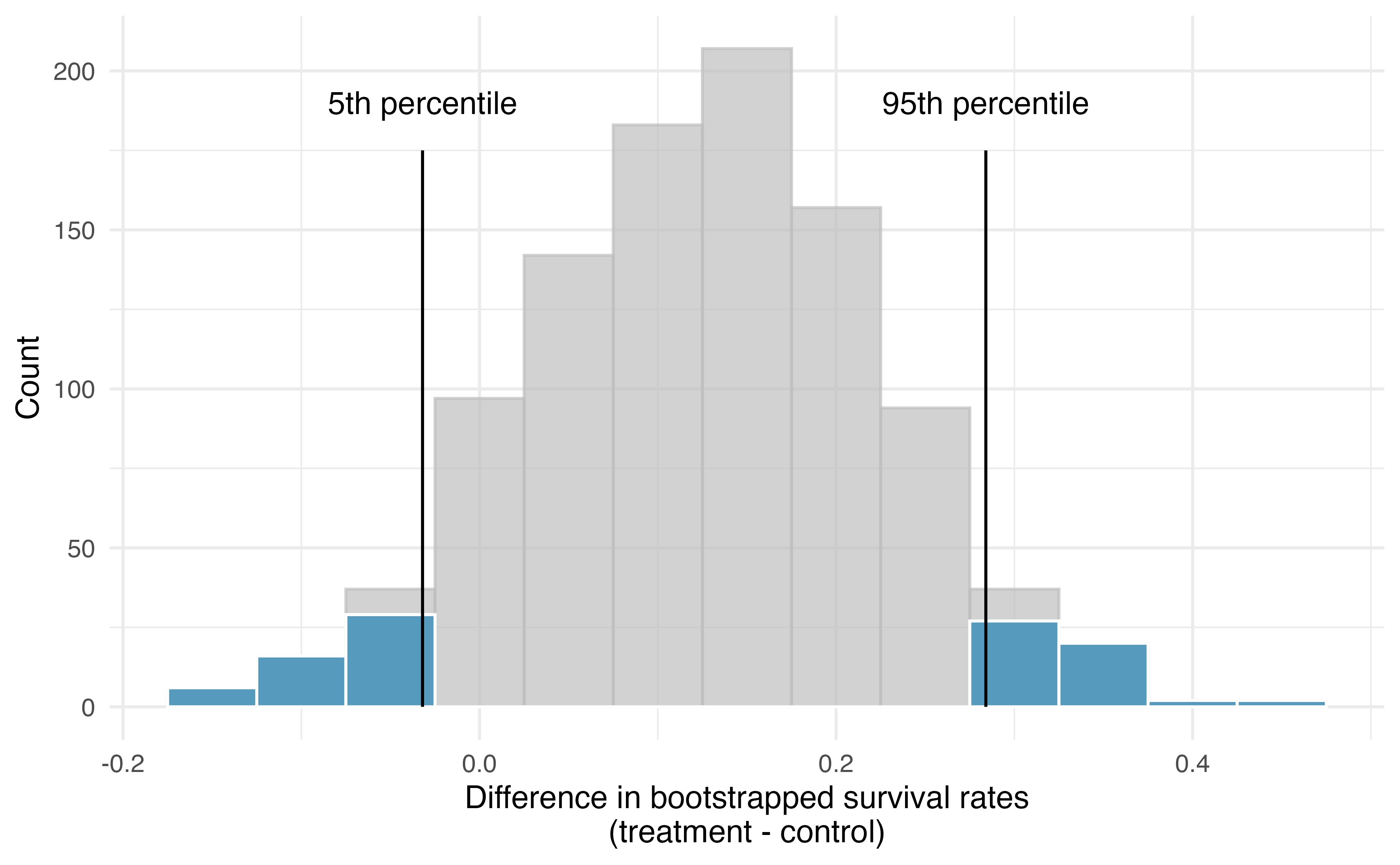
Alternatively, we can use the variability in the bootstrapped differences to calculate a standard error of the difference. The resulting interval is called the SE interval. Section 17.3 details the mathematical model for the standard error of the difference in sample proportions, but the bootstrap distribution typically does an excellent job of estimating the variability of the sampling distribution of the sample statistic.
\[ SE(\hat{p}_T - \hat{p}_C) \approx SE(\hat{p}_{T, boot} - \hat{p}_{C, boot}) = 0.098 \]
The variability of the difference in proportions was calculated in R using the sd() function, but any statistical software will calculate the standard deviation of the differences, here, the exact quantity we hope to approximate.
Note that we do not know the true distribution of \(\hat{p}_T - \hat{p}_C,\) so we will use a rough approximation to find a confidence interval for \(p_T - p_C.\) As seen in the bootstrap histograms, the shape of the distribution is roughly symmetric and bell-shaped. So for a rough approximation, we will apply the 67-95-99.7 rule which tells us that 95% of observed differences should be roughly no farther than 2 SE from the true parameter (difference in proportions). A 95% confidence interval for \(p_T - p_C\) is given by:
\[ \hat{p}_T - \hat{p}_C \pm 2 \cdot SE \rightarrow \ \ \ 14/40 - 11/50 \pm 2 \cdot 0.098 \ \ \ \rightarrow \ \ \ (-0.067, 0.327) \]
We are 95% confident that the true value of \(p_T - p_C\) is between -0.067 and 0.327. Again, the wide confidence interval that contains zero indicates that the study provides very little evidence about the effectiveness of blood thinners. For other percentages, e.g., a 90% bootstrap SE confidence interval, we will use quantiles given by the standard normal distribution, as seen in Section 13.2 and Figure 13.8.
17.2.4 What does 95% mean?
Recall that the goal of a confidence interval is to find a plausible range of values for a parameter of interest. The estimated statistic is not the value of interest, but it is typically the best guess for the unknown parameter. The confidence level (often 95%) is a number that takes a while to get used to. Surprisingly, the percentage does not describe the dataset at hand, it describes many possible datasets. One way to understand a confidence interval is to think about all the confidence intervals that you have ever made or that you will ever make as a scientist, the confidence level describes those intervals.
Figure 17.9 demonstrates a hypothetical situation in which 25 different studies are performed on the exact same population (with the same goal of estimating the true parameter value of \(p_1 - p_2 = 0.47).\) The study at hand represents one point estimate (a dot) and a corresponding interval. It is not possible to know whether the interval at hand is to the right of the unknown true parameter value (the black line) or to the left of that line. It is also impossible to know whether the interval captures the true parameter (is blue) or does not (is red). If we are making 95% intervals, then about 5% of the intervals we create over our lifetime will not capture the parameter of interest (e.g., will be red as in Figure 17.9). What we know is that over our lifetimes as scientists, about 95% of the intervals created and reported on will capture the parameter value of interest: thus the language “95% confident.”
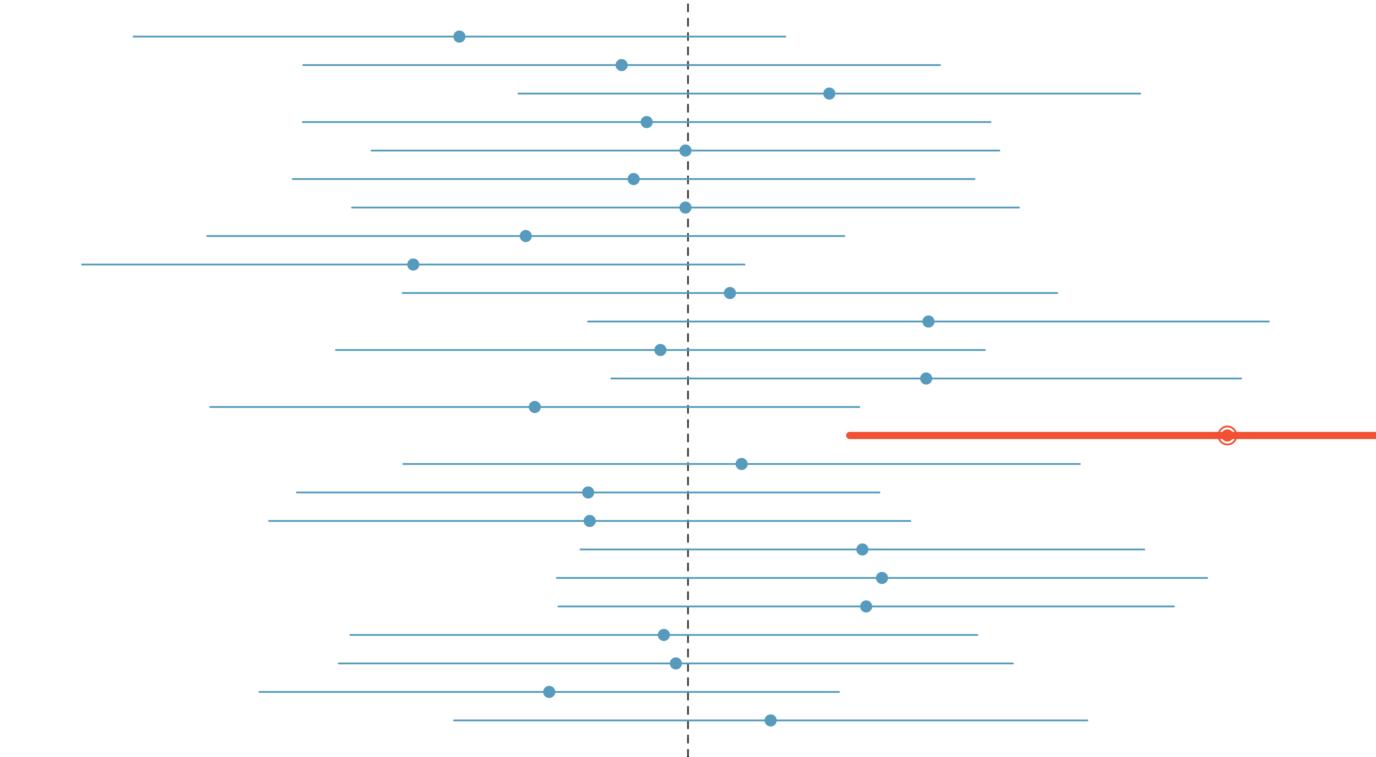
The choice of 95% or 90% or even 99% as a confidence level is admittedly somewhat arbitrary; however, it is related to the logic we used when deciding that a p-value should be declared as “discernible” if it is lower than 0.05 (or 0.10 or 0.01, respectively). Indeed, one can show mathematically, that a 95% confidence interval and a two-sided hypothesis test at a cutoff of 0.05 will provide the same conclusion when the same data and mathematical tools are applied for the analysis. A full derivation of the explicit connection between confidence intervals and hypothesis tests is beyond the scope of this text.
17.3 Mathematical model for the difference in proportions
17.3.1 Variability of the difference between two proportions
Like with \(\hat{p},\) the difference of two sample proportions \(\hat{p}_1 - \hat{p}_2\) can be modeled using a normal distribution when certain conditions are met. First, we require a broader independence condition, and secondly, the success-failure condition must be met by both groups.
Conditions for the sampling distribution of \(\hat{p}_1 -\hat{p}_2\) to be normal.
The difference \(\hat{p}_1 - \hat{p}_2\) can be modeled using a normal distribution when
- Independence (extended). The data are independent within and between the two groups. Generally this is satisfied if the data come from two independent random samples or if the data come from a randomized experiment.
- Success-failure condition. The success-failure condition holds for both groups, where we check successes and failures in each group separately. That is, we should have at least 10 successes and 10 failures in each of the two groups.
When these conditions are satisfied, the standard error of \(\hat{p}_1 - \hat{p}_2\) is:
\[SE(\hat{p}_1 - \hat{p}_2) = \sqrt{\frac{p_1(1-p_1)}{n_1} + \frac{p_2(1-p_2)}{n_2}}\]
where \(p_1\) and \(p_2\) represent the population proportions, and \(n_1\) and \(n_2\) represent the sample sizes.
Note that in most cases, the standard error is approximated using the observed data:
\[SE(\hat{p}_1 - \hat{p}_2) = \sqrt{\frac{\hat{p}_1(1-\hat{p}_1)}{n_1} + \frac{\hat{p}_2(1-\hat{p}_2)}{n_2}}\]
where \(\hat{p}_1\) and \(\hat{p}_2\) represent the observed sample proportions, and \(n_1\) and \(n_2\) represent the sample sizes.
Recall that the margin of error is defined by the standard error. The margin of error for \(\hat{p}_1 - \hat{p}_2\) can be directly obtained from \(SE(\hat{p}_1 - \hat{p}_2).\)
Margin of error for \(\hat{p}_1 - \hat{p}_2.\)
The margin of error is \(z^\star \times \sqrt{\frac{\hat{p}_1(1-\hat{p}_1)}{n_1} + \frac{\hat{p}_2(1-\hat{p}_2)}{n_2}}\) where \(z^\star\) is calculated from a specified percentile on the normal distribution.
17.3.2 Confidence interval for the difference between two proportions
We can apply the generic confidence interval formula for a difference of two proportions, where we use \(\hat{p}_1 - \hat{p}_2\) as the point estimate and substitute the \(SE\) formula:
\[ \begin{aligned} \text{point estimate} \ &\pm \ z^{\star} \ \times \ SE \\ (\hat{p}_1 - \hat{p}_2) \ &\pm \ z^{\star} \times \sqrt{\frac{\hat{p}_1(1-\hat{p}_1)}{n_1} + \frac{\hat{p}_2(1-\hat{p}_2)}{n_2}} \end{aligned} \]
Standard error of the difference in two proportions, \(\hat{p}_1 -\hat{p}_2.\)
When the conditions for the normal model are are met, the variability of the difference in proportions, \(\hat{p}_1 -\hat{p}_2,\) is well described by:
\[SE(\hat{p}_1 -\hat{p}_2) = \sqrt{\frac{\hat{p}_1(1-\hat{p}_1)}{n_1} + \frac{\hat{p}_2(1-\hat{p}_2)}{n_2}}\]
We reconsider the experiment for patients who underwent cardiopulmonary resuscitation (CPR) for a heart attack and were subsequently admitted to a hospital. These patients were randomly divided into a treatment group where they received a blood thinner or the control group where they did not receive a blood thinner. The outcome variable of interest was whether the patients survived for at least 24 hours. The results are shown in Table 14.2. Check whether we can model the difference in sample proportions using the normal distribution.
We first check for independence: since this is a randomized experiment, it seems reasonable to assume that the observations are idependent. Next, we check the success-failure condition for each group. We have at least 10 successes and 10 failures in each experiment arm (11, 14, 39, 26), so this condition is also satisfied. With both conditions satisfied, the difference in sample proportions can be reasonably modeled using a normal distribution for these data.
Create and interpret a 90% confidence interval of the difference for the survival rates in the CPR study.
We’ll use \(p_T\) for the survival rate in the treatment group and \(p_C\) for the control group:
\[\hat{p}_{T} - \hat{p}_{C} = \frac{14}{40} - \frac{11}{50} = 0.35 - 0.22 = 0.13\]
We use the standard error formula previously provided. As with the one-sample proportion case, we use the sample estimates of each proportion in the formula in the confidence interval context:
\[SE \approx \sqrt{\frac{0.35 (1 - 0.35)}{40} + \frac{0.22 (1 - 0.22)}{50}} = 0.095\]
For a 90% confidence interval, we use \(z^{\star} = 1.65:\)
\[ \begin{aligned} \text{point estimate} \ &\pm \ z^{\star} \ \times \ SE \\ 0.13 \ &\pm \ 1.65 \ \times \ 0.095 \\ (-0.027 \ &, \ 0.287) \end{aligned} \]
We are 90% confident that individuals receiving blood thinners have between a 2.7% less chance of survival to a 28.7% greater chance of survival than those in the control group. Because 0% is contained in the interval, we do not have enough information to say whether blood thinners help or harm heart attack patients who have been admitted after they have undergone CPR.
Note, the problem was set up as 90% to indicate that there was not a need for a high level of confidence (such a 95% or 99%). A lower degree of confidence increases potential for error, but it also produces a more narrow interval.
A 5-year experiment was conducted to evaluate the effectiveness of fish oils on reducing cardiovascular events, where each subject was randomized into one of two treatment groups (Manson et al. 2019). We’ll consider heart attack outcomes in the patients listed in Table 17.2.
Create a 95% confidence interval for the effect of fish oils on heart attacks for patients who are well-represented by those in the study. Also interpret the interval in the context of the study.2
| heart attack | no event | Total | |
|---|---|---|---|
| fish oil | 145 | 12788 | 12933 |
| placebo | 200 | 12738 | 12938 |
The fish_oil_18 data can be found in the openintro R package.
17.3.3 Hypothesis test for the difference between two proportions
The details for calculating a SE and for checking technical conditions are very similar to that of confidence intervals. However, when the null hypothesis is that \(p_1 - p_2 = 0,\) we use a special proportion called the pooled proportion to estimate the SE and to check the success-failure condition.
Use the pooled proportion when \(H_0\) is \(p_1 - p_2 = 0.\)
When the null hypothesis is that the proportions are equal, use the pooled proportion \((\hat{p}_{\textit{pool}})\) of successes to verify the success-failure condition and estimate the standard error:
\[\hat{p}_{\textit{pool}} = \frac{\text{number of successes}}{\text{number of cases}} = \frac{\hat{p}_1 n_1 + \hat{p}_2 n_2}{n_1 + n_2}\]
Here \(\hat{p}_1 n_1\) represents the number of successes in sample 1 because \(\hat{p}_1 = \frac{\text{number of successes in sample 1}}{n_1}.\)
Similarly, \(\hat{p}_2 n_2\) represents the number of successes in sample 2.
The test statistic for assessing two proportions is a Z.
The Z score is a ratio of how the two sample proportions differ as compared to the expected variability of difference between the proportions.
\[Z = \frac{(\hat{p}_1 - \hat{p}_2) - 0}{\sqrt{\hat{p}_{pool}(1-\hat{p}_{pool}) \bigg(\frac{1}{n_1} + \frac{1}{n_2} \bigg)}}\]
When the null hypothesis is true and the conditions are met, Z has a standard normal distribution. See the box below for calculation of the pooled proportion of successes.
Conditions:
- Independent observations
- Large samples: \((n_1 p_1 \geq 10\) and \(n_1 (1-p_1) \geq 10\) and \(n_2 p_2 \geq 10\) and \(n_2 (1-p_2) \geq 10)\)
- Check conditions using: \((n_1 \hat{p}_{\textit{pool}} \geq 10\) and \(n_1 (1-\hat{p}_{\textit{pool}}) \geq 10\) and \(n_2 \hat{p}_{\textit{pool}}\geq 10\) and \(n_2 (1-\hat{p}_{\textit{pool}}) \geq 10)\)
A mammogram is an X-ray procedure used to check for breast cancer. Whether mammograms should be used is part of a controversial discussion, and it’s the topic of our next example where we learn about 2-proportion hypothesis tests when \(H_0\) is \(p_1 - p_2 = 0\) (or equivalently, \(p_1 = p_2).\)
A 30-year study was conducted with nearly 90,000 participants who identified as female. During a 5-year screening period, each participant was randomized to one of two groups: in the first group, participants received regular mammograms to screen for breast cancer, and in the second group, participants received regular non-mammogram breast cancer exams. No intervention was made during the following 25 years of the study, and we’ll consider death resulting from breast cancer over the full 30-year period. Results from the study are summarized in Table 17.3.
If mammograms are much more effective than non-mammogram breast cancer exams, then we would expect to see additional deaths from breast cancer in the control group. On the other hand, if mammograms are not as effective as regular breast cancer exams, we would expect to see an increase in breast cancer deaths in the mammogram group.
| Treatment | Yes | No |
|---|---|---|
| control | 505 | 44,405 |
| mammogram | 500 | 44,425 |
Is this study an experiment or an observational study?3
Set up hypotheses to test whether there was a difference in breast cancer deaths in the mammogram and control groups.4
The research question describing mammograms is set up to address specific hypotheses (in contrast to a confidence interval for a parameter). In order to fully take advantage of the hypothesis testing structure, we assess the randomness under the condition that the null hypothesis is true (as we always do for hypothesis testing). Using the data from Table 17.3, we will check the conditions for using a normal distribution to analyze the results of the study using a hypothesis test.
\[ \begin{aligned} \hat{p}_{\textit{pool}} &= \frac {\text{number of patients who died from breast cancer in the entire study}} {\text{number of patients in the entire study}} \\ &= \frac{500 + 505}{500 + \text{44,425} + 505 + \text{44,405}} \\ &= 0.0112 \end{aligned} \]
This proportion is an estimate of the breast cancer death rate across the entire study, and it’s our best estimate of the proportions \(p_{MGM}\) and \(p_{C}\) if the null hypothesis is true that \(p_{MGM} = p_{C}.\) We will also use this pooled proportion when computing the standard error.
Is it reasonable to model the difference in proportions using a normal distribution in this study?
Because the patients were randomized, observations can be assumed to be independent, both within each group and between treatment groups. We also must check the success-failure condition for each group. Under the null hypothesis, the proportions \(p_{MGM}\) and \(p_{C}\) are equal, so we check the success-failure condition with our best estimate of these values under \(H_0,\) the pooled proportion from the two samples, \(\hat{p}_{\textit{pool}} = 0.0112:\)
\[ \begin{aligned} \hat{p}_{\textit{pool}} \times n_{MGM} &= 0.0112 \times \text{44,925} = 503\\ (1 - \hat{p}_{\textit{pool}}) \times n_{MGM} &= 0.9888 \times \text{44,925} = \text{44,422} \\ \hat{p}_{\textit{pool}} \times n_{C} &= 0.0112 \times \text{44,910} = 503\\ (1 - \hat{p}_{\textit{pool}}) \times n_{C} &= 0.9888 \times \text{44,910} = \text{44,407} \end{aligned} \]
The success-failure condition is satisfied since all values are at least 10. With both conditions satisfied, we can safely model the difference in proportions using a normal distribution.
In the previous example, the pooled proportion was used to check the success-failure condition5. In the next example, we see an additional place where the pooled proportion comes into play: the standard error calculation.
Compute the point estimate of the difference in breast cancer death rates in the two groups, and use the pooled proportion \(\hat{p}_{\textit{pool}} = 0.0112\) to calculate the standard error.
The point estimate of the difference in breast cancer death rates is
\[ \hat{p}_{MGM} - \hat{p}_{C} = \frac{500}{500 + 44,425} - \frac{505}{505 + 44,405} = 0.01113 - 0.01125 = -0.00012 \]
The breast cancer death rate in the mammogram group was 0.012% less than in the control group. Next, the standard error is calculated using the pooled proportion, \(\hat{p}_{\textit{pool}}:\)
\[SE = \sqrt{\frac{\hat{p}_{\textit{pool}}(1-\hat{p}_{\textit{pool}})}{n_{MGM}} + \frac{\hat{p}_{\textit{pool}}(1-\hat{p}_{\textit{pool}})}{n_{C}}}= 0.00070\]
Using the point estimate \(\hat{p}_{MGM} - \hat{p}_{C} = -0.00012\) and standard error \(SE = 0.00070,\) calculate a p-value for the hypothesis test and write a conclusion.
We first compute a test statistic and draw a picture:
\[Z = \frac{\text{point estimate} - \text{null value}}{SE} = \frac{-0.00012 - 0}{0.00070} = -0.17\]
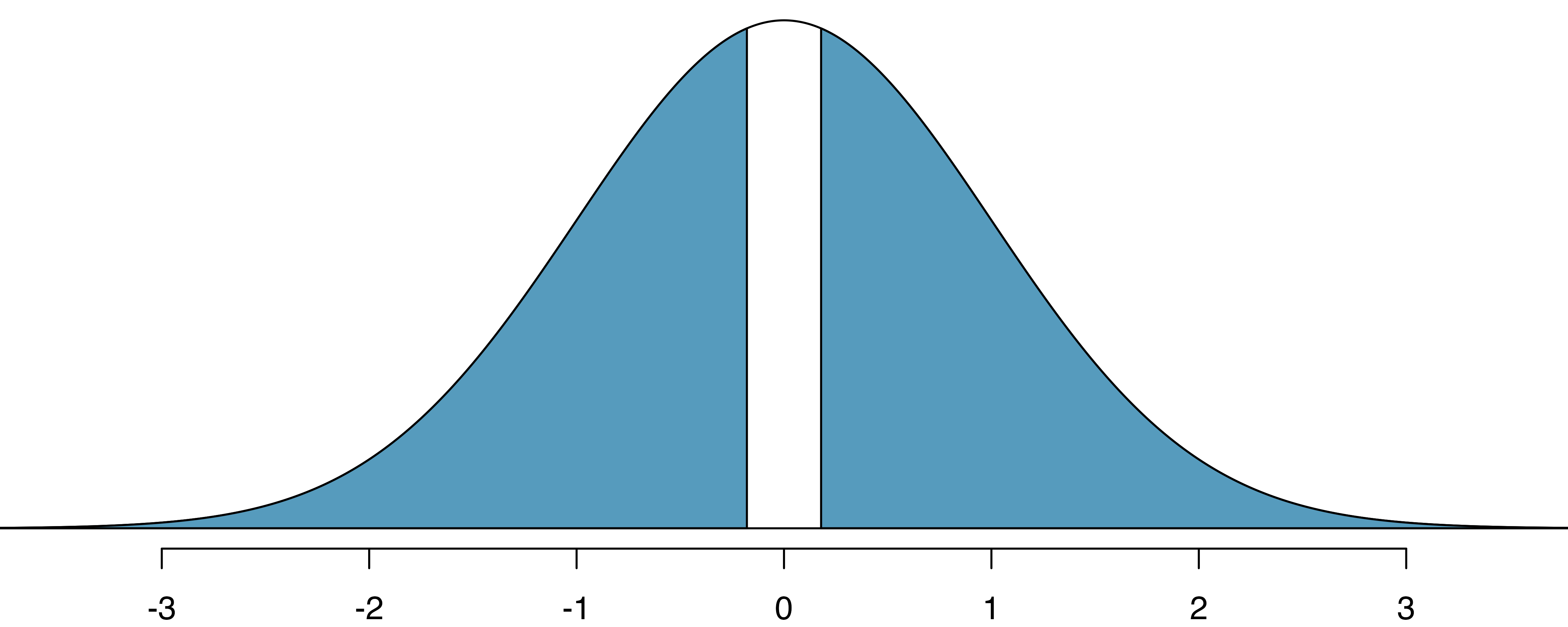
The lower tail area is 0.4325, which we double to get the p-value: 0.8650. Because this p-value is larger than 0.05, we do not reject the null hypothesis. That is, the difference in breast cancer death rates is likely to have occurred just by chance, if the null hypothesis is true. Thus, we do not observe benefits or harm from mammograms relative to a regular breast exam.
Can we conclude that mammograms have no benefits or harm? Here are a few considerations to keep in mind when reviewing the mammogram study as well as any other medical study:
- We do not reject the null hypothesis, which means we do not have sufficient evidence to conclude that mammograms reduce or increase breast cancer deaths.
- If mammograms are helpful or harmful, the data suggest the effect isn’t very large.
- Are mammograms more or less expensive than a non-mammogram breast exam? If one option is much more expensive than the other and does not offer clear benefits, then we should lean towards the less expensive option.
- The study’s authors also found that mammograms led to over-diagnosis of breast cancer, which means some breast cancers were found (or thought to be found) but that these cancers would not cause symptoms during patients’ lifetimes. That is, something else would kill the patient before breast cancer symptoms appeared. This means some patients may have been treated for breast cancer unnecessarily, and this treatment is another cost to consider. It is also important to recognize that over-diagnosis can cause unnecessary physical or emotional harm to patients.
These considerations highlight the complexity around medical care and treatment recommendations. Experts and medical boards who study medical treatments use considerations like those above to provide their best recommendation based on the current evidence.
17.4 Chapter review
17.4.1 Summary
When the parameter of interest is the difference in population proportions across two groups, randomization tests, bootstrapping, and mathematical modeling can be applied. For confidence intervals, bootstrapping from each group separately will provide a sampling distribution for the difference in sample proportions; the mathematical model shows a similar distributional shape as long as the sample size is large enough to fulfill the success-failure conditions and so that the data are representative of the entire population. Keep in mind that some datasets will produce a confidence interval which does not capture the true parameter, this is the nature of variability! Over your lifetime, about 95% of the confidence intervals you create will capture the parameter of interest, and about 5% won’t. For hypothesis testing, repeated randomization of the explanatory variable creates a null distribution of differences in sample proportions that could have occurred under the null hypothesis. Randomization and the mathematical model will have similar null distributions, as long as the sample size is large enough to fulfill the success-failure conditions.
17.4.2 Terms
The terms introduced in this chapter are presented in Table 17.4. If you’re not sure what some of these terms mean, we recommend you go back in the text and review their definitions. You should be able to easily spot them as bolded text.
| percentile interval | pooled proportion | SE interval |
| point estimate | SE difference in proportions | Z score two proportions |
17.5 Exercises
Answers to odd-numbered exercises can be found in Appendix A.17.
-
Disaggregating Asian American tobacco use, hypothesis testing. Understanding cultural differences in tobacco use across different demographic groups can lead to improved health care education and treatment. A recent study disaggregated tobacco use across Asian American ethnic groups including Asian-Indian (n = 4,373), Chinese (n = 4,736), and Filipino (n = 4,912), in comparison to non-Hispanic Whites (n = 275,025). The number of current smokers in each group was reported as Asian-Indian (n = 223), Chinese (n = 279), Filipino (n = 609), and non-Hispanic Whites (n = 50,880). (Rao et al. 2021)
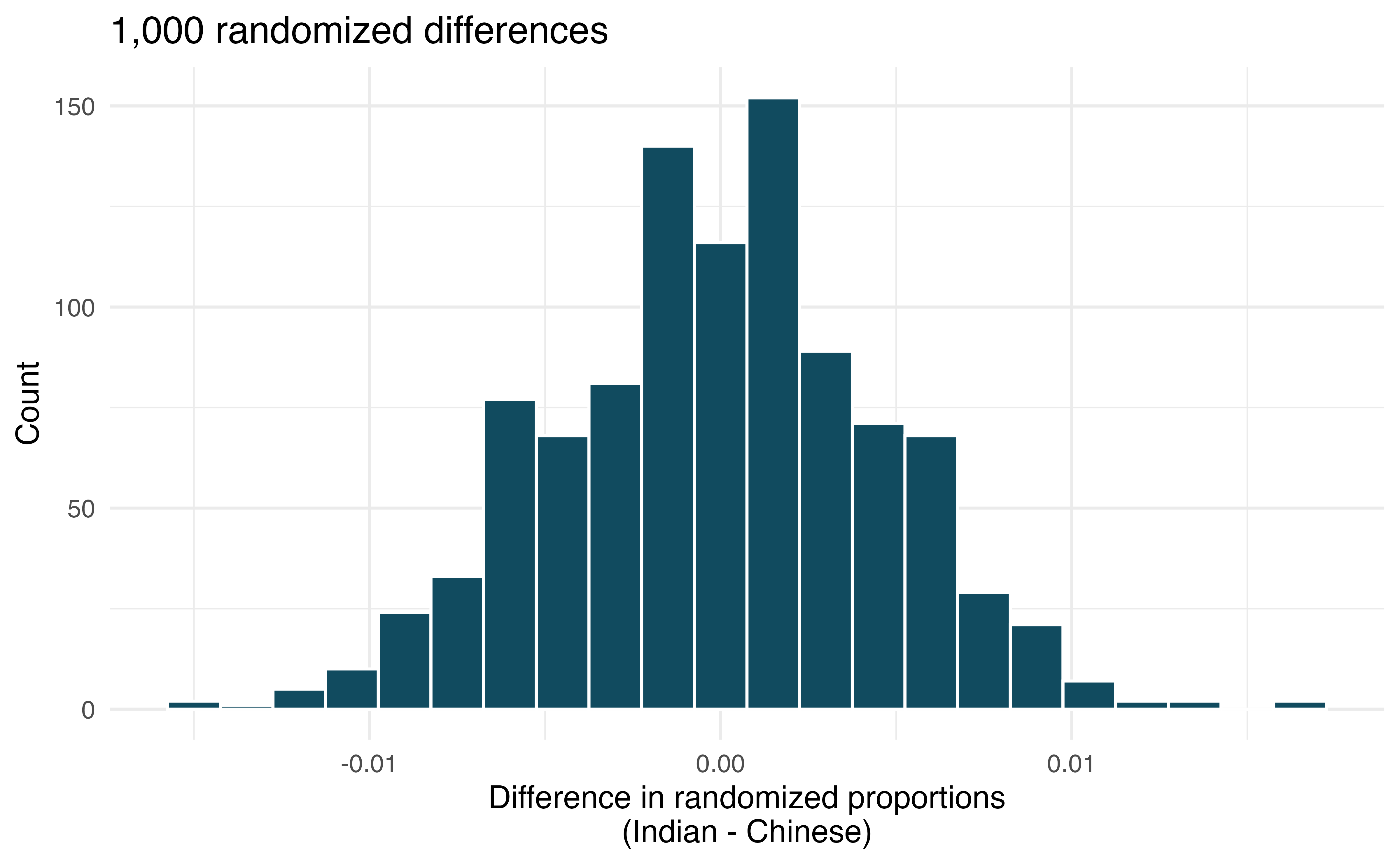
To determine whether the proportion of Asian-Indian Americans who are current smokers is different from the proportion of Chinese Americans who are smokers, a randomization simulation was performed.
In both words and symbols provide the parameter and statistic of interest for this study. Do you know the numerical value of either the parameter or statistic of interest? If so, provide the numerical value.
The histogram above provides the sampling distribution (under randomization) for \(\hat{p}_{Asian-Indian} - \hat{p}_{Chinese}\) under repeated null randomizations (\(\hat{p}\) is the proportion in the sample who are current smokers). Estimate the standard error of \(\hat{p}_{Asian-Indian} - \hat{p}_{Chinese}\) based on the randomization histogram.
Consider the hypothesis test to determine if there is a difference in proportion of Asian-Indian Americans as compared to Chinese Americans who are current smokers. Write out the null and alternative hypotheses, estimate a p-value using the randomization histogram, and conclude the test in the context of the problem.
-
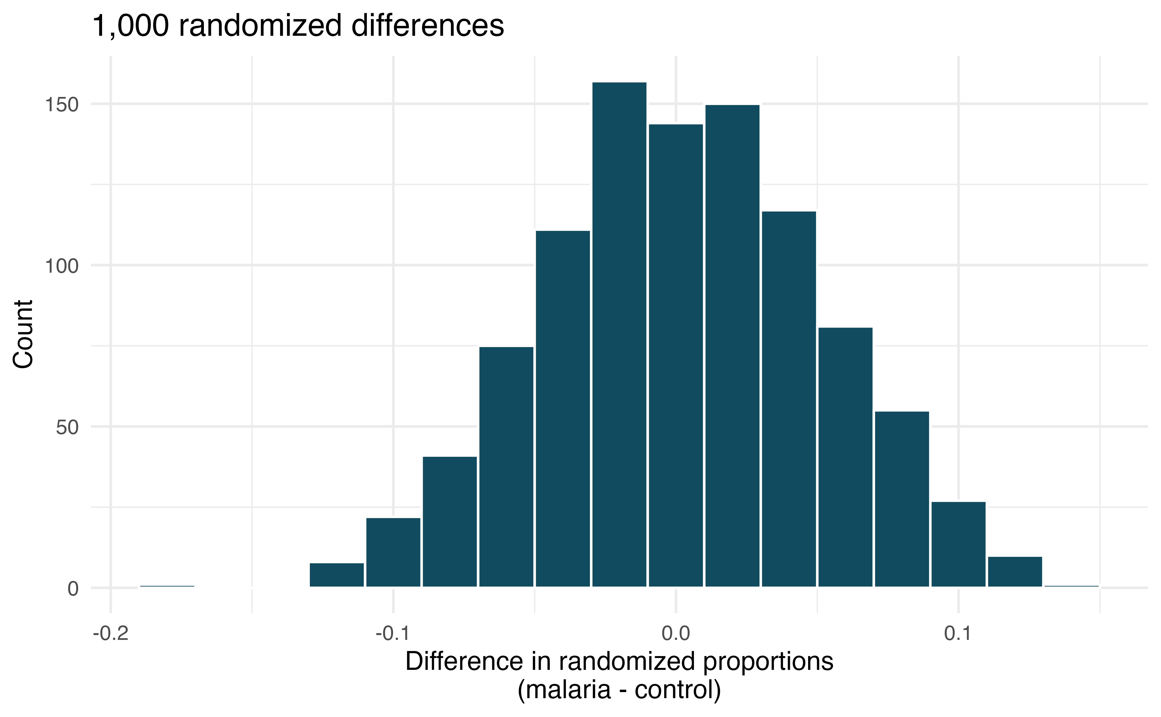
Malaria vaccine effectiveness, hypothesis test. With no currently licensed vaccines to inhibit malaria, good news was welcomed with a recent study reporting long-awaited vaccine success for children in Burkina Faso. With 450 children randomized to either one of two different doses of the malaria vaccine or a control vaccine, 89 of 292 malaria vaccine and 106 out of 147 control vaccine children contracted malaria within 12 months after the treatment. (Datoo et al. 2021)
In both words and symbols provide the parameter and statistic of interest for this study. Do you know the numerical value of either the parameter or statisic of interest? If so, provide the numerical value.
The histogram above provides the sampling distribution (under randomization) for \(\hat{p}_{malaria} - \hat{p}_{control}\) under repeated null randomizations (\(\hat{p}\) is the proportion of children in the sample who contracted malaria). Estimate the standard error of \(\hat{p}_{malaria} - \hat{p}_{control}\) based on the randomization histogram.
Consider the hypothesis test constructed to show a lower proportion of children contracting malaria on the malaria vaccine as compared to the control vaccine. Write out the null and alternative hypotheses, estimate a p-value using the randomization histogram, and conclude the test in the context of the problem.
-
Disaggregating Asian American tobacco use, confidence interval. Based on a study on the degree to which smoking practices differ across ethnic groups. a confidence interval for the difference in current smoking status for Filipino versus Chinese Americans is desired. (Rao et al. 2021)
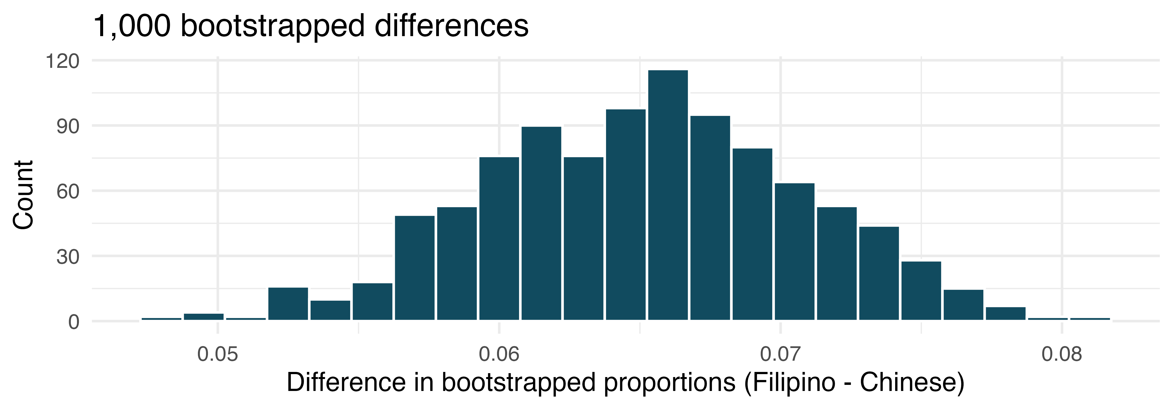
Consider the bootstrap distribution of difference in sample proportions of current smokers (Filipino Americans minus Chinese Americans) in 1,000 bootstrap repetitions as above. Estimate the standard error of the difference in sample proportions, as seen in the histogram.
Using the standard error from the bootstrap distribution, find a 95% bootstrap SE confidence interval for the true difference in proportion of current smokers (Filipino Americans minus Chinese Americans) in the population. Interpret the interval in the context of the problem.
Using the entire bootstrap distribution, find a 95% bootstrap percentile confidence interval for the true difference in proportion of current smokers (Filipino Americans minus Chinese Americans) in the population. Interpret the interval in the context of the problem.
-
Malaria vaccine effectiveness, confidence interval. With no currently licensed vaccines to inhibit malaria, good news was welcomed with a recent study reporting long-awaited vaccine success for children in Burkina Faso. With 450 children randomized to either one of two different doses of the malaria vaccine or a control vaccine, 89 of 292 malaria vaccine and 106 out of 147 control vaccine children contracted malaria within 12 months after the treatment. (Datoo et al. 2021)
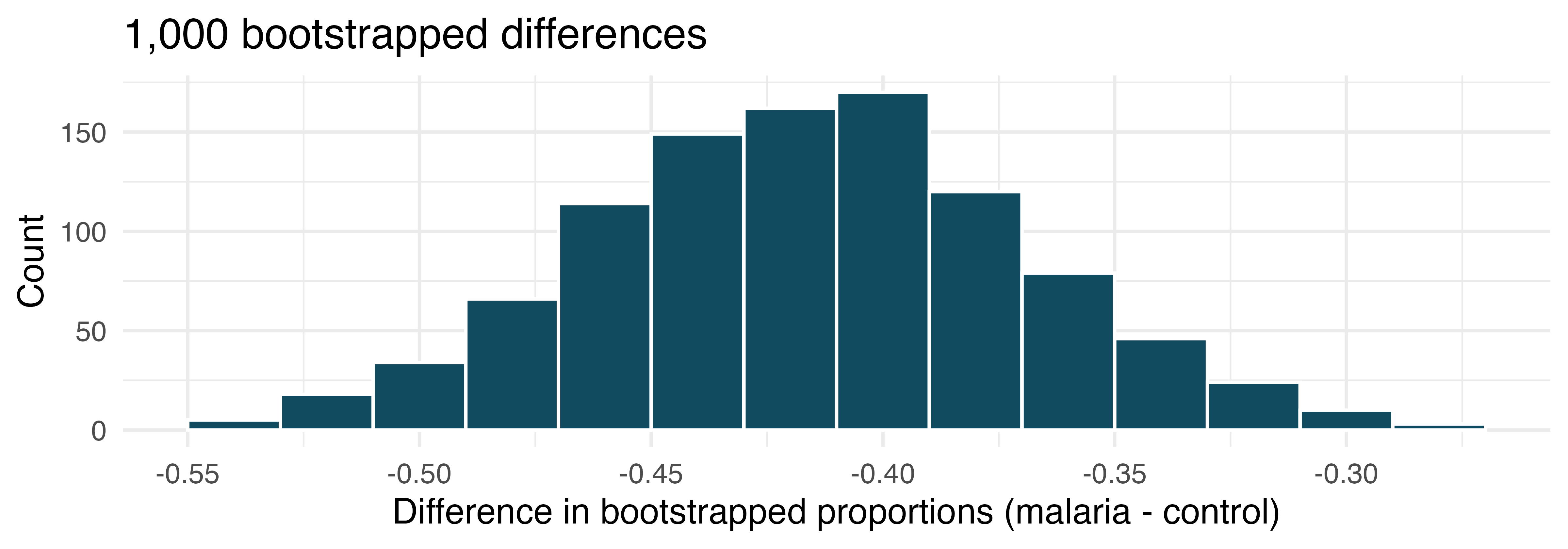
Consider the bootstrap distribution of difference in sample proportions of children who contracted malaria (malaria vaccine minus control vaccine) in 1000 bootstrap repetitions as above. Estimate the standard error of the difference in sample proportions, as seen in the histogram.
Using the standard error from the bootstrap distribution, find a 95% bootstrap SE confidence interval for the true difference in proportion of children who contract malaria (malaria vaccine minus control vaccine) in the population. Interpret the interval in the context of the problem.
Using the entire bootstrap distribution, find a 95% bootstrap percentile confidence interval for the true difference in proportion of children who contract malaria (malaria vaccine minus control vaccine) in the population. Interpret the interval in the context of the problem.
-
COVID-19 and degree completion. A 2021 Gallup poll surveyed 3,941 students pursuing a bachelor’s degree and 2,064 students pursuing an associate degree (students were not randomly selected but were weighted so as to represent a random selection of currently enrolled US college students). The poll found that 51% of the bachelor’s degree students and 44% of associate degree students said that the COVID-19 pandemic will negatively impact their ability to complete the degree. (Gallup 2021)
Below are two histograms generated with different computational approaches (both use 1,000 repetitions) to research questions which could be asked of these data. One of the histograms can be used to do a randomization test on whether the proportions of bachelor’s and associate students who think the COVID-19 pandemic will negatively impact their ability to complete the degree. The other histogram is a bootstrap distribution used to quantify the difference in the proportions of bachelor’s and associate’s students who feel this way.
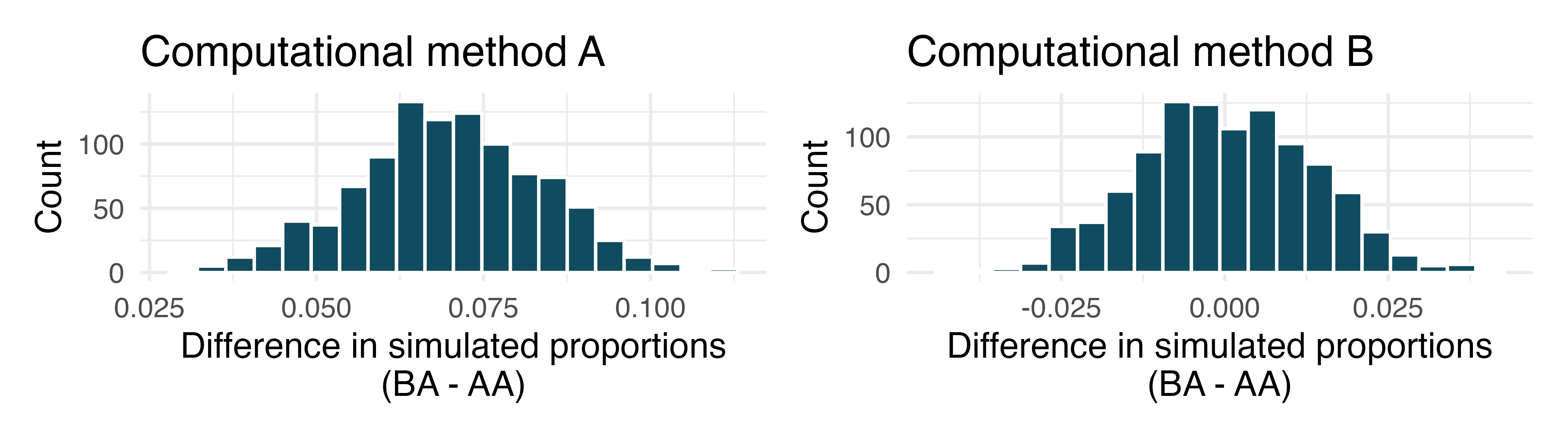
Are the center and standard error of the two graphs approximately the same? Explain.
Write a research question that can be addressed using the histogram generated with computational method A.
Write a research question that can addressed using the histogram generated with computational method B.
-
Renewable energy. A 2021 Gallup poll surveyed 5,447 randomly sampled US adults who are Republican (or Republican leaning) and 7,962 who are Democrats (or Democrat leaning). 31% of Republicans and 81% of Democrats said “government regulations are necessary to encourage businesses and consumers to rely more on renewable energy sources”. (Gallup 2021)
Below are two histograms generated with different computational approaches (both use 1,000 repetitions) to research questions which could be asked of these data. One of the histograms can be used to do a randomization test on whether the proportions of Republicans and Democrats who think government regulations are necessary to encourage businesses and consumers to rely more on renewable energy sources are different. The other histogram is a bootstrap distribution used to quantify the difference in the proportions of Republicans and Democrats who agree with this statement.
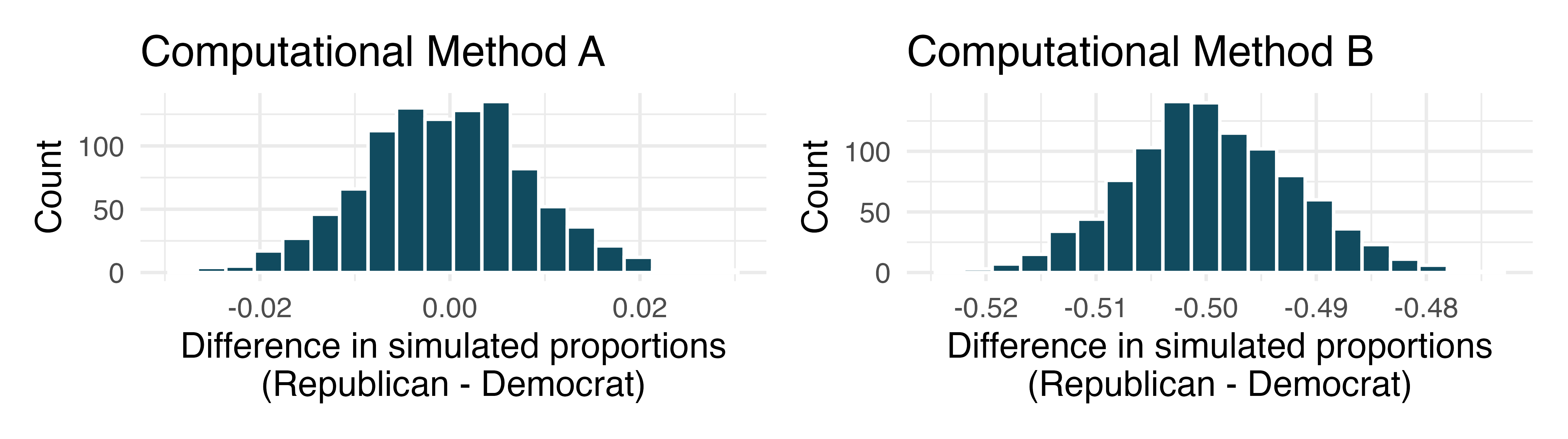
Are the center and standard error of the two graphs approximately the same? Explain.
Write a research question that can addressed using the histogram generated with computational method A.
Write a research question that can addressed using the histogram generated with computational method B.
-
HIV in sub-Saharan Africa. In July 2008 the US National Institutes of Health announced that it was stopping a clinical study early because of unexpected results. The study population consisted of HIV-infected women in sub-Saharan Africa who had been given single dose Nevaripine (a treatment for HIV) while giving birth, to prevent transmission of HIV to the infant. The study was a randomized comparison of continued treatment of a woman (after successful childbirth) with Nevaripine vs Lopinavir, a second drug used to treat HIV. 240 women participated in the study; 120 were randomized to each of the two treatments. Twenty-four weeks after starting the study treatment, each woman was tested to determine if the HIV infection was becoming worse (an outcome called virologic failure). Twenty-six of the 120 women treated with Nevaripine experienced virologic failure, while 10 of the 120 women treated with the other drug experienced virologic failure. (Lockman et al. 2007)
Create a two-way table presenting the results of this study.
State appropriate hypotheses to test for difference in virologic failure rates between treatment groups.
Complete the hypothesis test and state an appropriate conclusion. (Reminder: Verify any necessary conditions for the test.)
-
Supercommuters. The fraction of workers who are considered “supercommuters”, because they commute more than 90 minutes to get to work, varies by state. Suppose the 1% of Nebraska residents and 6% of New York residents are supercommuters. Now suppose that we plan a study to survey 1000 people from each state, and we will compute the sample proportions \(\hat{p}_{NE}\) for Nebraska and \(\hat{p}_{NY}\) for New York.
What is the associated mean and standard deviation of \(\hat{p}_{NE}\) in repeated samples of size 1000?
What is the associated mean and standard deviation of \(\hat{p}_{NY}\) in repeated samples of size 1000?
Calculate and interpret the mean and standard deviation associated with the difference in sample proportions for the two groups, \(\hat{p}_{NY} - \hat{p}_{NE}\) in repeated samples of 1000 in each group.
How are the standard deviations from parts (a), (b), and (c) related?
-
National Health Plan. A Kaiser Family Foundation poll for US adults in 2019 found that 79% of Democrats, 55% of Independents, and 24% of Republicans supported a generic “National Health Plan”. There were 347 Democrats, 298 Republicans, and 617 Independents surveyed. 79% of 347 Democrats and 55% of 617 Independents support a National Health Plan. (Kaiser Family Foundation 2019)
Calculate a 95% confidence interval for the difference between the proportion of Democrats and Independents who support a National Health Plan \((p_{D} - p_{I})\), and interpret it in this context. We have already checked conditions for you.
True or false: If we had picked a random Democrat and a random Independent at the time of this poll, it is more likely that the Democrat would support the National Health Plan than the Independent.
- Sleep deprivation, CA vs. OR, confidence interval. According to a report on sleep deprivation by the Centers for Disease Control and Prevention, the proportion of California residents who reported insufficient rest or sleep during each of the preceding 30 days is 8.0%, while this proportion is 8.8% for Oregon residents. These data are based on simple random samples of 11,545 California and 4,691 Oregon residents. Calculate a 95% confidence interval for the difference between the proportions of Californians and Oregonians who are sleep deprived and interpret it in context of the data. (CDC 2008)
-
Gender pay gap in medicine. A study examined the average pay for men and women entering the workforce as doctors for 21 different positions. (Lo Sasso et al. 2011)
If each gender was equally paid, then we would expect about half of those positions to have men paid more than women and women would be paid more than men in the other half of positions. Write appropriate hypotheses to test this scenario.
Men were, on average, paid more in 19 of those 21 positions. Complete a hypothesis test using your hypotheses from part (a).
-
Sleep deprivation, CA vs. OR, hypothesis test. A CDC report on sleep deprivation rates shows that the proportion of California residents who reported insufficient rest or sleep during each of the preceding 30 days is 8.0%, while this proportion is 8.8% for Oregon residents. These data are based on simple random samples of 11,545 California and 4,691 Oregon residents.
Conduct a hypothesis test to determine if these data provide strong evidence that the rate of sleep deprivation is different for the two states. (Reminder: Check conditions)
It is possible the conclusion of the test in part (a) is incorrect. If this is the case, what type of error was made?
-
Is yawning contagious? An experiment conducted by the MythBusters, a science entertainment TV program on the Discovery Channel, tested if a person can be subconsciously influenced into yawning if another person near them yawns. 50 people were randomly assigned to two groups: 34 to a group where a person near them yawned (treatment) and 16 to a group where there wasn’t a person yawning near them (control). The visualization below displays how many participants yawned in each group.6
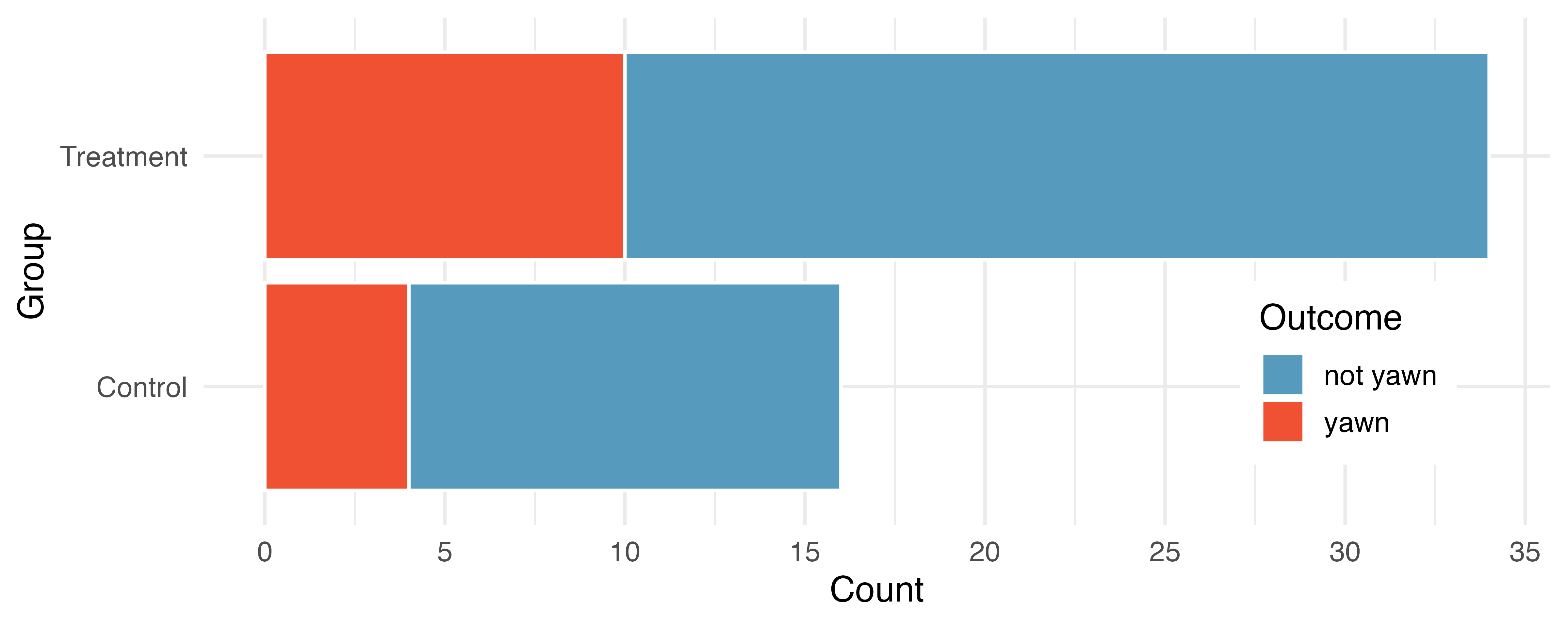
Suppose we are interested in estimating the difference in yawning rates between the control and treatment groups using a confidence interval. Explain why we cannot construct such an interval using the normal approximation. What might go wrong if we constructed the confidence interval despite this problem?
-
Heart transplant success. The Stanford University Heart Transplant Study was conducted to determine whether an experimental heart transplant program increased lifespan. Each patient entering the program was officially designated a heart transplant candidate, meaning that he was gravely ill and might benefit from a new heart. Patients were randomly assigned into treatment and control groups. Patients in the treatment group received a transplant, and those in the control group did not. The visualization below displays how many patients survived and died in each group.7 (Turnbull et al. 1974)
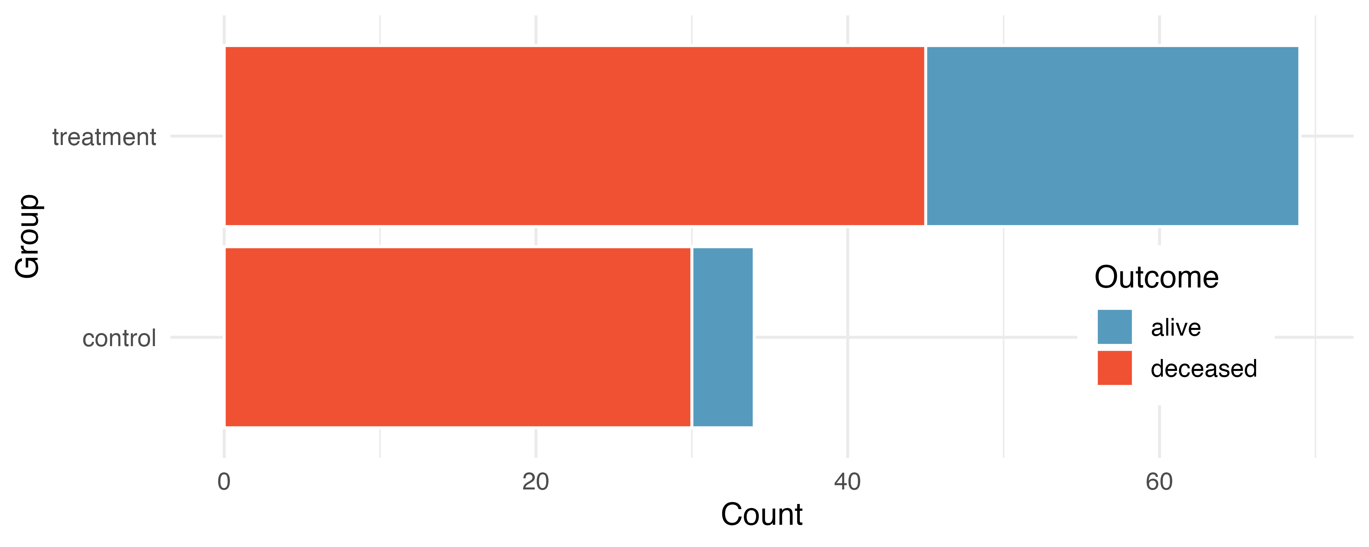
Suppose we are interested in estimating the difference in survival rate between the control and treatment groups using a confidence interval. Explain why we cannot construct such an interval using the normal approximation. What might go wrong if we constructed the confidence interval despite this problem?
-
Government shutdown. The United States federal government shutdown of 2018–2019 occurred from December 22, 2018 until January 25, 2019, a span of 35 days. A Survey USA poll of 614 randomly sampled Americans during this time period reported that 48% of those who make less than $40,000 per year and 55% of those who make $40,000 or more per year said the government shutdown has not at all affected them personally. A 95% confidence interval for \((p_\text{$<$40K} - p_\text{$\ge$40K})\), where \(p\) is the proportion of those who said the government shutdown has not at all affected them personally, is (-0.16, 0.02). Based on this information, determine if the following statements are true or false, and explain your reasoning if you identify the statement as false. (Survey USA 2019)
At the 5% discernibility level, the data provide convincing evidence of a real difference in the proportion who are not affected personally between Americans who make less than $40,000 annually and Americans who make $40,000 annually.
We are 95% confident that 16% more to 2% fewer Americans who make less than $40,000 per year are not at all personally affected by the government shutdown compared to those who make $40,000 or more per year.
A 90% confidence interval for \((p_\text{$<$40K} - p_\text{$\ge$40K})\) would be wider than the \((-0.16, 0.02)\) interval.
A 95% confidence interval for \((p_\text{$\ge$40K} - p_\text{$<$40K})\) is (-0.02, 0.16).
-
Online harassment. A Pew Research poll asked US adults aged 18-29 and 30-49 whether they have personally experienced harassment online. A 95% confidence interval for the difference between the proportions of 18-29 year-olds and 30-49 year-olds who have personally experienced harassment online \((p_{18-29} - p_{30-49})\) was calculated to be (0.115, 0.185). Based on this information, determine if the following statements are true or false, and explain your reasoning for each statement you identify as false. (Pew Research Center 2021)
We are 95% confident that the true proportion of 18-29 year-olds who have personally experienced harassment online is 11.5% to 18.5% lower than the true proportion of 30-49 year-olds who have personally experienced harassment online.
We are 95% confident that the true proportion of 18-29 year-olds who have personally experienced harassment online is 11.5% to 18.5% higher than the true proportion of 30-49 year-olds who have personally experienced harassment online.
95% of random samples will produce 95% confidence intervals that include the true difference between the population proportions of 18-29 year-olds and 30-49 year-olds who have personally experienced harassment online.
We can conclude that there is a discernible difference between the proportions of 18-29 year-olds and 30-49 year-olds who have personally experienced harassment online is too large to plausibly be due to chance, if in fact there is no difference between the two proportions.
The 90% confidence interval for \((p_{18-29} - p_{30-49})\) cannot be calculated with only the information given in this exercise.
-
Decision errors and comparing proportions I. In the following research studies, conclusions were made based on the data provided. It is always possible that the analysis conclusion could be wrong, although we will almost never actually know if an error has been made or not. For each study conclusion, specify which of a Type I or Type II error could have been made, and state the error in the context of the problem.
The malaria vaccine was seen to be effective at lowering the rate of contracting malaria (when compared to the control vaccine).
In the US population, Asian-Indian Americans and Chinese Americans are not observed to have different proportions of current smokers.
There is no evidence to claim a difference in the proportion of Americans who are not affected personally by a government shutdown when comparing Americans who make less than $40,000 annually and Americans who make $40,000 annually.
-
Decision errors and comparing proportions II. In the following research studies, conclusions were made based on the data provided. It is always possible that the analysis conclusion could be wrong, although we will almost never actually know if an error has been made or not. For each study conclusion, specify which of a Type I or Type II error could have been made, and state the error in the context of the problem.
Of registered voters in California, the proportion who report not knowing enough to voice an opinion on whether they support off shore drilling is different across those who have a college degree and those who do not.
In comparing Californians and Oregonians, there is no evidence to support a difference in the proportion of each who are sleep deprived.
- Active learning. A teacher wanting to increase the active learning component of her course is concerned about student reactions to changes she is planning to make. She conducts a survey in her class, asking students whether they believe more active learning in the classroom (hands on exercises) instead of traditional lecture will helps improve their learning. She does this at the beginning and end of the semester and wants to evaluate whether students’ opinions have changed over the semester. Can she used the methods we learned in this chapter for this analysis? Explain your reasoning.
- An apple a day keeps the doctor away. A physical education teacher at a high school wanting to increase awareness on issues of nutrition and health asked her students at the beginning of the semester whether they believed the expression “an apple a day keeps the doctor away”. 40% of the students responded yes. Throughout the semester she started each class with a discussion of a study highlighting positive effects of eating more fruits and vegetables. She conducted the same apple-a-day survey at the end of the semester, and this time 60% of the students responded yes. Can she used a two-proportion method from this section for this analysis? Explain your reasoning.
-
Malaria vaccine effectiveness, effect size. A randomized controlled trial on malaria vaccine effectiveness randomly assigned 450 children intro either one of two different doses of the malaria vaccine or a control vaccine. 89 of 292 malaria vaccine and 106 out of 147 control vaccine children contracted malaria within 12 months after the treatment. (Datoo et al. 2021)
Recall that in order to reject the null hypothesis that the two vaccines (malaria and control) are equivalent, we’d need the sample proportion to be about 2 standard errors below the hypothesized value of zero.
Say that the true difference (in the population) is given as \(\delta,\) the sample sizes are the same in both groups \((n_{malaria} = n_{control}),\) and the true proportion who contract malaria on the control vaccine is \(p_{control} = 0.7.\) If you ran your own study (in the future), how likely is it that you would get a difference in sample proportions that was sufficiently far from zero that you could reject under each of the conditions below. (Hint: Use the mathematical model.)
\(\delta = -0.1\) and \(n_{malaria} = n_{control} = 20\)
\(\delta = -0.4\) and \(n_{malaria} = n_{control} = 20\)
\(\delta = -0.1\) and \(n_{malaria} = n_{control} = 100\)
\(\delta = -0.4\) and \(n_{malaria} = n_{control} = 100\)
What can you conclude about values of \(\delta\) and the sample size?
-
Diabetes and unemployment. A Gallup poll surveyed Americans about their employment status and whether they have diabetes. The survey results indicate that 1.5% of the 47,774 employed (full or part time) and 2.5% of the 5,855 unemployed 18-29 year-olds have diabetes. (Gallup 2012)
Create a two-way table presenting the results of this study.
State appropriate hypotheses to test for difference in proportions of diabetes between employed and unemployed Americans.
The sample difference is about 1%. If we completed the hypothesis test, we would find that the p-value is very small (about 0), meaning the difference is statistically discernible. Use this result to explain the difference between statistically discernible and practically important findings.
The study is an experiment, as patients were randomly assigned an experiment group. Since this is an experiment, the results can be used to evaluate a causal relationship between blood thinner use after CPR and whether patients survived.↩︎
Because the patients were randomized, the subjects are independent, both within and between the two groups. The success-failure condition is also met for both groups as all counts are at least 10. This satisfies the conditions necessary to model the difference in proportions using a normal distribution. Compute the sample proportions \((\hat{p}_{\text{fish oil}} = 0.0112,\) \(\hat{p}_{\text{placebo}} = 0.0155),\) point estimate of the difference \((0.0112 - 0.0155 = -0.0043),\) and standard error \(SE = \sqrt{\frac{0.0112 \times 0.9888}{12933} + \frac{0.0155 \times 0.9845}{12938}},\) \(SE = 0.00145.\) Next, plug the values into the general formula for a confidence interval, where we’ll use a 95% confidence level with \(z^{\star} = 1.96:\) \(-0.0043 \pm 1.96 \times 0.00145 = (-0.0071, -0.0015).\) We are 95% confident that fish oils decreases heart attacks by 0.15 to 0.71 percentage points (off of a baseline of about 1.55%) over a 5-year period for subjects who are similar to those in the study. Because the interval is entirely below 0, and the treatment was randomly assigned the data provide strong evidence that fish oil supplements reduce heart attacks in patients like those in the study.↩︎
This is an experiment. Patients were randomized to receive mammograms or a standard breast cancer exam. We will be able to make causal conclusions based on this study.↩︎
\(H_0:\) the breast cancer death rate for patients screened using mammograms is the same as the breast cancer death rate for patients in the control, \(p_{MGM} - p_{C} = 0.\) \(H_A:\) the breast cancer death rate for patients screened using mammograms is different than the breast cancer death rate for patients in the control, \(p_{MGM} - p_{C} \neq 0.\)↩︎
For an example of a two-proportion hypothesis test that does not require the success-failure condition to be met, see Section 17.1.↩︎
The
yawndata used in this exercise can be found in the openintro R package.↩︎The
heart_transplantdata used in this exercise can be found in the openintro R package.↩︎