English

16 Inference for a single proportion

Focusing now on statistical inference for categorical data, we will revisit many of the foundational aspects of hypothesis testing from Chapter 11.

The three data structures we detail are one binary variable, summarized using a single proportion; two binary variables, summarized using a difference of two proportions; and two categorical variables, summarized using a two-way table. When appropriate, each of the data structures will be analyzed using the three methods from Chapter 11, Chapter 12, and Chapter 13: randomization test, bootstrapping, and mathematical models, respectively.

As we build on the inferential ideas, we will visit new foundational concepts in statistical inference. For example, we will cover the conditions for when a normal model is appropriate; the two different error rates in hypothesis testing; and choosing the confidence level for a confidence interval.

We encountered inference methods for a single proportion in Chapter 12, exploring point estimates and confidence intervals. In this section, we’ll do a review of these topics and how to choose an appropriate sample size when collecting data for single proportion contexts.

Note that there is only one variable being measured in a study which focuses on one proportion. For each observational unit, the single variable is measured as either a success or failure (e.g., “surgical complication” vs. “no surgical complication”). Because the nature of the research question at hand focuses on only a single variable, there is not a way to randomize the variable across a different (explanatory) variable. For this reason, we will not use randomization as an analysis tool when focusing on a single proportion. Instead, we will apply bootstrapping techniques to test a given hypothesis, and we will also revisit the associated mathematical models.

16.1 Bootstrap test for a proportion

The bootstrap simulation concept when $H_0$ is true is similar to the ideas used in the case studies presented in Chapter 12 where we bootstrapped without an assumption about $H_0.$ Because we will be testing a hypothesized value of $p$ (referred to as $p_0),$ the bootstrap simulation for hypothesis testing has a fantastic advantage that it can be used for any sample size (a huge benefit for small samples, a nice alternative for large samples).

We expand on the medical consultant example from Section 12.1, but instead of finding an interval estimate for the true complication rate, we test a specific claim.

16.1.1 Observed data

Recall the set-up for the example: People providing an organ for donation sometimes seek the help of a special “medical consultant”. These consultants assist the patient in all aspects of the surgery, with the goal of reducing the possibility of complications during the medical procedure and recovery. Patients might choose a consultant based in part on the historical complication rate of the consultant’s clients. One consultant tried to attract patients by noting the average complication rate for liver donor surgeries in the US is about 10%, but her clients have only had 3 complications in the 62 liver donor surgeries she has facilitated. She claims this is strong evidence that her work meaningfully contributes to reducing complications (and therefore she should be hired!).

Using the data, is it possible to assess the consultant’s claim that her complication rate is less than 10%?

No. The claim is that there is a causal connection, but the data are observational. Patients who hire this medical consultant may have lower complication rates for other reasons.

While it is not possible to assess this causal claim, it is still possible to test for an association using these data. For this question we ask, could the low complication rate of $\hat{p} = 0.0484$ have simply occurred by chance, if her complication rate does not differ from the US standard rate?

Write out hypotheses in both plain and statistical language to test for the association between the consultant’s work and the true complication rate, $p,$ for the consultant’s clients.¹

Because, as it turns out, the conditions of working with the normal distribution are not met (see Section 16.2), the uncertainty associated with the sample proportion should not be modeled using the normal distribution, as doing so would underestimate the uncertainty associated with the sample statistic. However, we would still like to assess the hypotheses from the previous Guided Practice in absence of the normal framework. To do so, we need to evaluate the possibility of a sample value $(\hat{p})$ as far below the null value, $p_0 = 0.10$ as what was observed. The deviation of the sample value from the hypothesized parameter is usually quantified with a p-value.

The p-value is computed based on the null distribution, which is the distribution of the test statistic if the null hypothesis is true. Supposing the null hypothesis is true, we can compute the p-value by identifying the probability of observing a test statistic that favors the alternative hypothesis at least as strongly as the observed test statistic. Here we will use a bootstrap simulation to calculate the p-value.

16.1.2 Variability of the statistic

We want to identify the sampling distribution of the test statistic $(\hat{p})$ if the null hypothesis was true. In other words, we want to see the variability we can expect from sample proportions if the null hypothesis was true. Then we plan to use this information to decide whether there is enough evidence to reject the null hypothesis.

Under the null hypothesis, 10% of liver donors have complications during or after surgery. Suppose this rate was really no different for the consultant’s clients (for all the consultant’s clients, not just the 62 previously measured). If this was the case, we could simulate 62 clients to get a sample proportion for the complication rate from the null distribution. Simulating observations using a hypothesized null parameter value is often called a parametric bootstrap simulation, but we will refer to it descriptively as “simulating under the null hypothesis claim.”

Similar to the process described in Chapter 12, each client can be simulated using a bag of marbles with 10% red marbles and 90% white marbles. Sampling a marble from the bag (with 10% red marbles) is one way of simulating whether a patient has a complication if the true complication rate is 10%. If we select 62 marbles and then compute the proportion of patients with complications in the simulation, $\hat{p}_{sim1},$ then the resulting sample proportion is a sample from the null distribution.

There were 5 simulated cases with a complication and 57 simulated cases without a complication, i.e., $\hat{p}_{sim1} = 5/62 = 0.081.$

Is this one simulation enough to determine whether we should reject the null hypothesis?

No. To assess the hypotheses, we need to see a distribution of many values of $\hat{p}_{sim},$ not just a single draw from this sampling distribution.

16.1.3 Observed statistic vs. null statistics

One simulation isn’t enough to get a sense of the null distribution; many simulation studies are needed. Roughly 10,000 seems sufficient. However, paying someone to simulate 10,000 studies by hand is a waste of time and money. Instead, simulations are typically programmed into a computer, which is much more efficient.

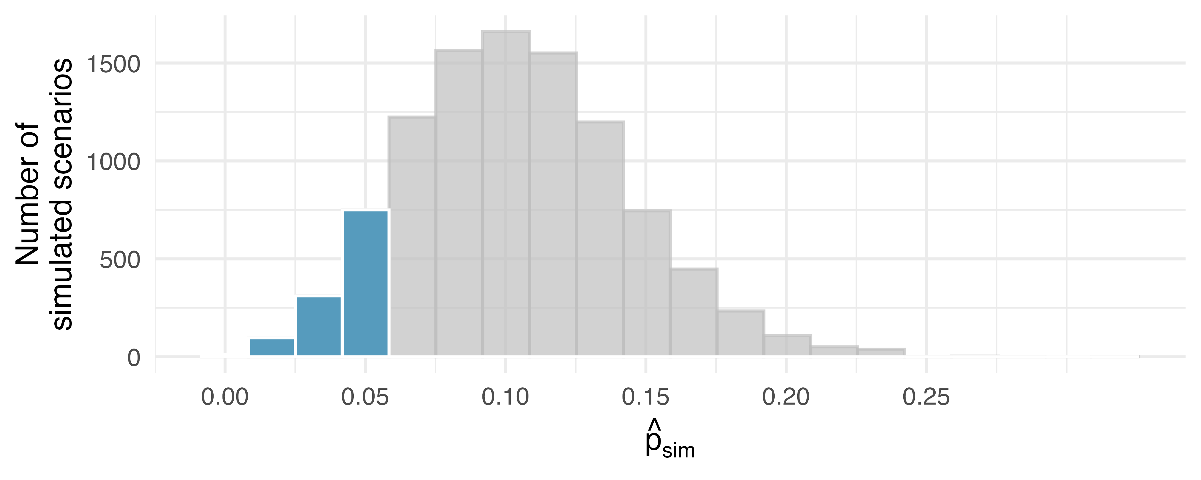
Figure 16.1 shows the results of 10,000 simulated studies. The proportions that are equal to or less than $\hat{p} = 0.0484$ are shaded. The shaded areas represent sample proportions under the null distribution that provide at least as much evidence as $\hat{p}$ favoring the alternative hypothesis. There were 1170 simulated sample proportions with $\hat{p}_{sim} \leq 0.0484.$ We use these to construct the null distribution’s left-tail area and find the p-value:

\[\text{left tail area} = \frac{\text{Number of observed simulations with }\hat{p}_{sim} \leq \text{ 0.0484}}{10000}\]

Of the 10,000 simulated $\hat{p}_{sim},$ 1170 were equal to or smaller than $\hat{p}.$ Since the hypothesis test is one-sided, the estimated p-value is equal to this tail area: 0.117.

Histogram of 10,000 simulated sample proportions, from the null distribution, where the true proportion is 0.1. The left tail, representing the p-value for the hypothesis test, is colored in blue. — Figure 16.1: The null distribution for $\hat{p},$ created from 10,000 simulated studies. The left tail, representing the p-value for the hypothesis test is colored in blue.

Because the estimated p-value is 0.117, which is larger than the discernibility level 0.05, we cannot reject the null hypothesis. Explain what this means in plain language in the context of the problem.²

Does the conclusion in the previous Guided Practice imply the consultant is good at their job? Explain.³

Null distribution of $\hat{p}$ with bootstrap simulation.

Regardless of the statistical method chosen, the p-value is always derived by analyzing the null distribution of the test statistic. The normal model poorly approximates the null distribution for $\hat{p}$ (the sample proportion) when the success-failure condition is not satisfied. As a substitute, we can generate the null distribution using simulated sample proportions and use this distribution to compute the tail area, i.e., the p-value.

In the previous Guided Practice, the p-value is estimated. It is not exact because the simulated null distribution itself is only a close approximation of the sampling distribution of the sample statistic. An exact p-value can be generated using the binomial distribution, but that method will not be covered in this text.

16.2 Mathematical model for a proportion

16.2.1 Conditions

In Section 13.2, we introduced the normal distribution and showed how it can be used as a mathematical model to describe the variability of a statistic. There are conditions under which a sample proportion $\hat{p}$ is well modeled with a normal distribution. When the observations are independent and the sample size is sufficiently large, the normal model will describe the sampling distribution of the sample proportion quite well; when the observations violate the conditions, the normal model can be inaccurate. Particularly, it can underestimate the variability of the sample proportion.

Sampling distribution of $\hat{p}.$

The sampling distribution for $\hat{p}$ (the sample proportion) based on a sample of size $n$ from a population with a true proportion $p$ is nearly normal when:

The sample’s observations are independent, e.g., are from a simple random sample.
We expected to see at least 10 successes and 10 failures in the sample, i.e., $np\geq10$ and $n(1-p)\geq10.$ This is called the success-failure condition.

When these conditions are met, then the sampling distribution of $\hat{p}$ is nearly normal with mean $p$ and standard error of $\hat{p}$ as $SE = \sqrt{\frac{\ \hat{p}(1-\hat{p})\ }{n}}.$

Recall that the margin of error is defined by the standard error. The margin of error for $\hat{p}$ can be directly obtained from $SE(\hat{p}).$

Margin of error for $\hat{p}.$

The margin of error is $z^\star \times \sqrt{\frac{\ \hat{p}(1-\hat{p})\ }{n}}$ where $z^\star$ is calculated from a specified percentile on the normal distribution.

Typically we do not know the true proportion $p,$ so we substitute some value to check conditions and estimate the standard error. For confidence intervals, the sample proportion $\hat{p}$ is used to check the success-failure condition and compute the standard error. For hypothesis tests, typically the null value – that is, the proportion claimed in the null hypothesis – is used in place of $p.$

The independence condition is a more nuanced requirement. When it isn’t met, it is important to understand how and why it is violated. For example, there exist no statistical methods available to truly correct the inherent biases of data from a convenience sample. On the other hand, if we took a cluster sample (see Section 2.1.5), the observations wouldn’t be independent, but suitable statistical methods are available for analyzing the data (but they are beyond the scope of even most second or third courses in statistics).

In the examples based on large sample theory, we modeled $\hat{p}$ using the normal distribution. Why is this not appropriate for the case study on the medical consultant?

The independence assumption may be reasonable if each of the surgeries is from a different surgical team. However, the success-failure condition is not satisfied. Under the null hypothesis, we would anticipate seeing $62 \times 0.10 = 6.2$ complications, not the 10 required for the normal approximation.

While this book is scoped to well-constrained statistical problems, do remember that this is just the first book in what is a large library of statistical methods that are suitable for a very wide range of data and contexts.

16.2.2 Confidence interval for a proportion

A confidence interval provides a range of plausible values for the parameter $p,$ and when $\hat{p}$ can be modeled using a normal distribution, the confidence interval for $p$ takes the form $\hat{p} \pm z^{\star} \times SE.$ We have seen $\hat{p}$ to be the sample proportion. The value $z^{\star}$ determines the confidence level (previously set to be 1.96) and will be discussed in detail in the examples following. The value of the standard error, $SE,$ depends heavily on the sample size.

Standard error of one proportion, $\hat{p}.$

When the conditions are met so that the distribution of $\widehat{p}$ (the sample proportion) is nearly normal, the variability of a single proportion, $\widehat{p}$ is well described by:

\[SE(\hat{p}) = \sqrt{\frac{p(1-p)}{n}}\]

Note that we almost never know the true value of $p$ (the population probability or proportion). A more helpful formula to use is:

\[ SE(\hat{p}) \approx \sqrt{\frac{(\mbox{best guess of }p)(1 - \mbox{best guess of }p)}{n}} \]

For hypothesis testing, we use $p_0$ (the proportion specified in the null hypothesis) as the best guess of $p.$ For confidence intervals, we use $\widehat{p}$ as the best guess of $p.$

Consider taking many polls of registered voters (i.e., random samples) of size 300 asking them if they support legalized marijuana. It is suspected that about 2/3 of all voters support legalized marijuana. To understand how the sample proportion $(\hat{p})$ would vary across the samples, calculate the standard error of $\hat{p}.$⁴

16.2.3 Variability of the sample proportion

A simple random sample of 826 payday loan borrowers was surveyed to better understand their interests around regulation and costs. 70% of the responses supported new regulations on payday lenders.

Is it reasonable to model the distribution of $\hat{p}$ using a normal distribution?
Estimate the standard error of $\hat{p}.$
Construct a 95% confidence interval for $p,$ the proportion of payday borrowers who support increased regulation for payday lenders.

The data are a random sample, so it is reasonable to assume that the observations are independent and representative of the population of interest. We also must check the success-failure condition, using $\hat{p}$ in place of $p$ when computing a confidence interval. Since both values are at least 10, we can use the normal distribution to model $\hat{p}.$

\[ \begin{aligned} \text{Support: } n p & \approx 826 \times 0.70 = 578\\ \text{Not: } n (1 - p) & \approx 826 \times (1 - 0.70) = 248 \end{aligned} \] 2. Because $p$ is unknown and the standard error is for a confidence interval, use $\hat{p}$ in place of $p$ in the formula.

\[SE = \sqrt{\frac{p(1-p)}{n}} \approx \sqrt{\frac{0.70 (1 - 0.70)} {826}} = 0.016.\]

Using $\hat{p} = 0.70$, $z^{\star} = 1.96$ for a 95% confidence interval, and the standard error $SE = 0.016$ from the previous Guided Practice, the confidence interval is

\[ \begin{aligned} \text{point estimate} \ &\pm \ z^{\star} \times \ SE \\ 0.70 \ &\pm \ 1.96 \ \times \ 0.016 \\ (0.669 \ &, \ 0.731) \end{aligned} \] We are 95% confident that the true proportion of payday borrowers who supported regulation at the time of the poll was between 0.669 and 0.731.

Constructing a confidence interval for a single proportion.

There are three steps to constructing a confidence interval for $p$ (the true population proportion or probability).

Check if it seems reasonable to assume the observations are independent and check the success-failure condition using $\hat{p}$ (the sample proportion). If the conditions are met, the sampling distribution of $\hat{p}$ may be well-approximated by the normal model.
Calculate the standard error using $\hat{p}$ instead of $p$.
Apply the general confidence interval formula.

For additional one-proportion confidence interval examples, see Section 12.3.

16.2.4 Changing the confidence level

Suppose we want to consider confidence intervals where the confidence level is somewhat higher than 95%: perhaps we would like a confidence level of 99%. Think back to the analogy about trying to catch a fish: if we want to be more sure that we will catch the fish, we should use a wider net. To create a 99% confidence level, we must also widen our 95% interval. On the other hand, if we want an interval with lower confidence, such as 90%, we could make our original 95% interval slightly slimmer.

The 95% confidence interval structure provides guidance in how to make intervals with new confidence levels. Below is a general 95% confidence interval for a point estimate that comes from a nearly normal distribution:

\[ \text{point estimate} \ \pm \ 1.96 \ \times \ SE \]

There are three components to this interval: the point estimate, “1.96”, and the standard error. The choice of $1.96 \times SE$ was based on capturing 95% of the data since the estimate is within 1.96 standard errors of the true value about 95% of the time. 1.96 corresponds to the 95% confidence level.

If $X$ is a normally distributed random variable, how often will $X$ be within 2.58 standard deviations of the mean?⁵

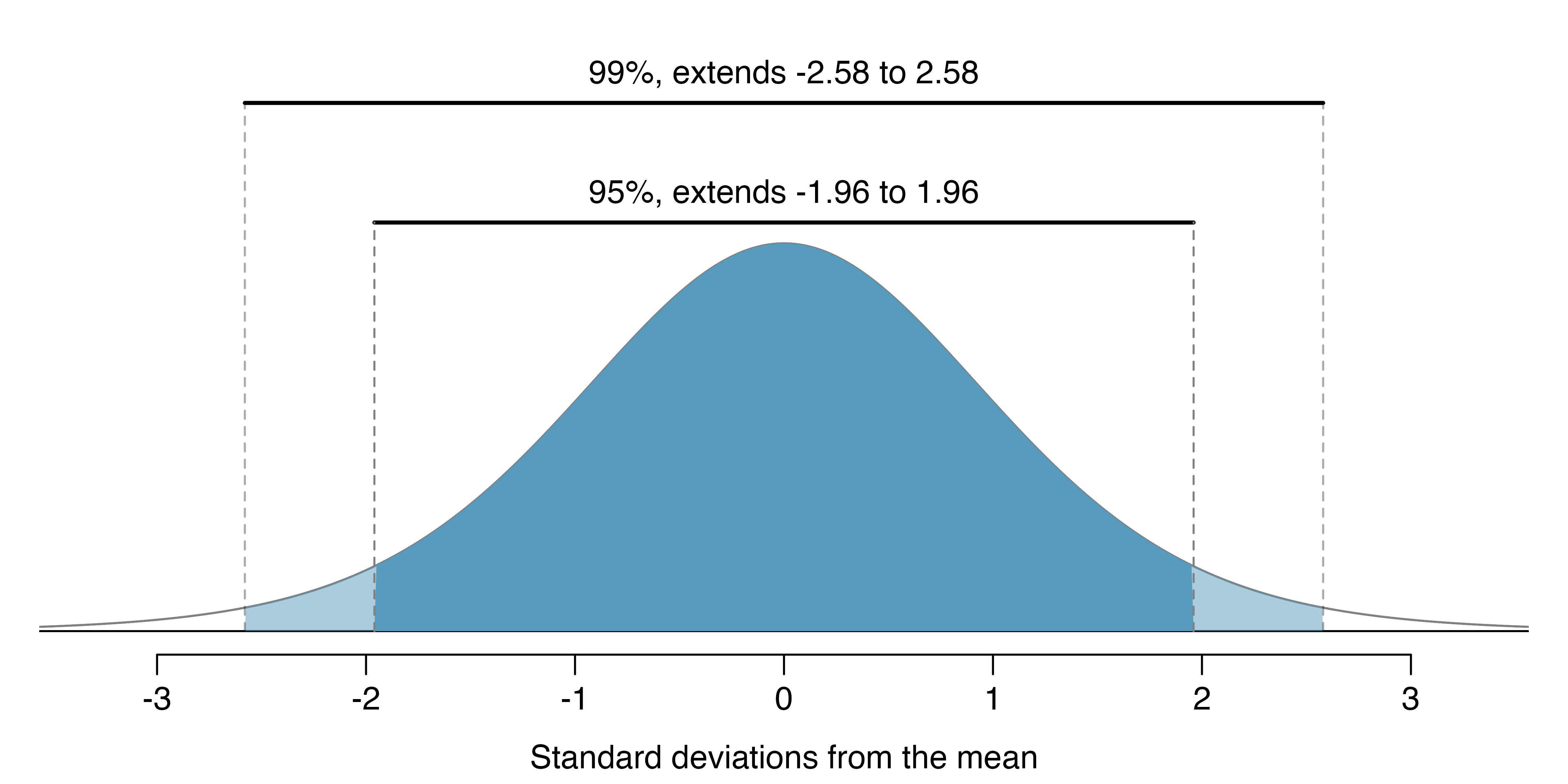
A normal curve with 99% of the area between negative z star and positive z star. The area between negative z star and positive z star increases as $| z star becomes larger. If the confidence level is 99 percent, we choose z star such that 99 percent of the normal curve is between negative z star and positive z star, which corresponds to 0.5 percent in the lower tail and 0.5 percent in the upper tail. The z star value is 2.58. — Figure 16.2: The area between -$z^{\star}$ and $z^{\star}$ increases as $|z^{\star}|$ becomes larger. If the confidence level is 99%, we choose $z^{\star}$ such that 99% of the normal curve is between -$z^{\star}$ and $z^{\star},$ which corresponds to 0.5% in the lower tail and 0.5% in the upper tail: $z^{\star}=2.58.$

To create a 99% confidence interval, change 1.96 in the 95% confidence interval formula to be $2.58.$ The previous Guided Practice highlights that 99% of the time a normal random variable will be within 2.58 standard deviations of its mean. This approach – using the Z scores in the normal model to compute confidence levels – is appropriate when the point estimate is associated with a normal distribution and we can properly compute the standard error. Thus, the formula for a 99% confidence interval is:

\[ \text{point estimate} \ \pm \ 2.58 \ \times \ SE \]

The normal approximation is crucial to the precision of the $z^\star$ confidence intervals (in contrast to the bootstrap percentile confidence intervals). When the normal model is not a good fit, we will use alternative distributions that better characterize the sampling distribution or we will use bootstrapping procedures.

Create a 99% confidence interval for the impact of the stent on the risk of stroke using the data from Section 1.1. The point estimate is 0.090, and the standard error is $SE = 0.028.$ It has been verified for you that the point estimate can reasonably be modeled by a normal distribution.⁶

Mathematical model confidence interval for any confidence level.

If the point estimate follows the normal model with standard error $SE,$ then a confidence interval for the population parameter is

\[ \text{point estimate} \ \pm \ z^{\star} \ \times \ SE \]

where $z^{\star}$ corresponds to the confidence level selected.

Figure 16.2 provides a picture of how to identify $z^{\star}$ based on a confidence level. We select $z^{\star}$ so that the area between -$z^{\star}$ and $z^{\star}$ in the normal model corresponds to the confidence level.

Previously, we found that implanting a stent in the brain of a patient at risk for a stroke increased the risk of a stroke. The study estimated a 9% increase in the number of patients who had a stroke, and the standard error of this estimate was about $SE = 2.8%.$ Compute a 90% confidence interval for the effect.⁷

16.2.5 Hypothesis test for a proportion

One possible regulation for payday lenders is that they would be required to do a credit check and evaluate debt payments against the borrower’s finances. We would like to know: would borrowers support this form of regulation?

Set up hypotheses to evaluate whether borrowers have a majority support for this type of regulation.⁸

To apply the normal distribution framework in the context of a hypothesis test for a proportion, the independence and success-failure conditions must be satisfied. In a hypothesis test, the success-failure condition is checked using the null proportion: we verify $np_0$ and $n(1-p_0)$ are at least 10, where $p_0$ is the null value.

The test statistic for assessing a single proportion is a Z.

The Z score is a ratio of how the sample proportion differs from the hypothesized proportion $(p_0)$ as compared to the expected variability of the $\hat{p}$ (sample proportion) values.

\[ Z = \frac{\hat{p} - p_0}{\sqrt{p_0(1 - p_0)/n}} \]

When the null hypothesis is true and the conditions are met, Z has a standard normal distribution.

Conditions:

independent observations
large samples $(n p_0 \geq 10$ and $n (1-p_0) \geq 10)$

Do payday loan borrowers support a regulation that would require lenders to pull their credit report and evaluate their debt payments? From a random sample of 826 borrowers, 51% said they would support such a regulation. Is it reasonable to use a normal distribution to model $\hat{p}$ for a hypothesis test here?⁹

Mathematical model hypothesis test for a proportion.

Set up hypotheses and verify the conditions using the null value, $p_0,$ to ensure $\hat{p}$ (the sample proportion) is nearly normal under $H_0.$ If the conditions hold, calculate the standard error, again using $p_0,$ and show the p-value in a drawing. Lastly, compute the p-value and evaluate the hypotheses.

For additional one-proportion hypothesis test examples, see Section 11.3.

Using the hypotheses and data from the previous Guided Practices, evaluate whether the poll on lending regulations provides convincing evidence that a majority of payday loan borrowers support a new regulation that would require lenders to pull credit reports and evaluate debt payments.

With hypotheses already set up and conditions checked, we can move onto calculations. The standard error in the context of a one-proportion hypothesis test is computed using the null value, $p_0:$

\[ SE = \sqrt{\frac{p_0 (1 - p_0)}{n}} = \sqrt{\frac{0.5 (1 - 0.5)}{826}} = 0.017 \]

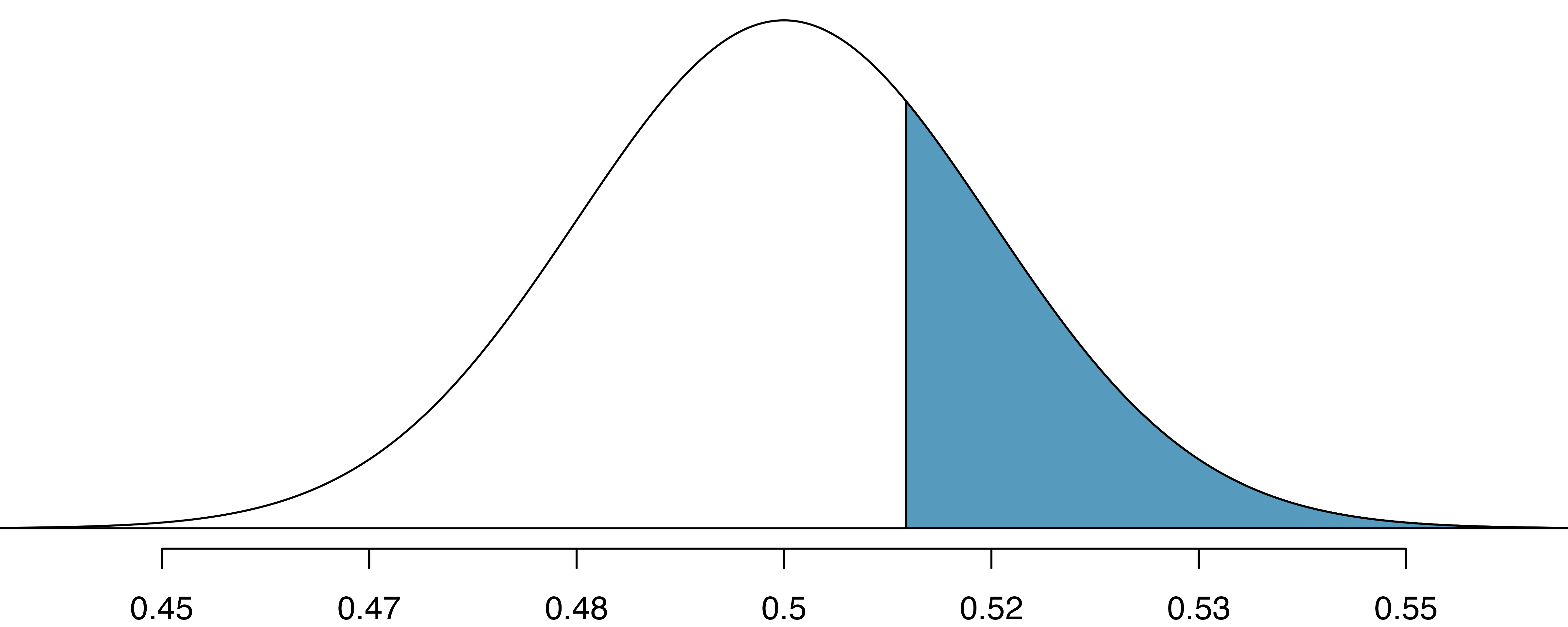
A picture of the normal model is shown below with the p-value represented by the shaded region.

A normal curve centered at 0.5 with a standard deviation of 0.017. The area to the right of 0.51 is shaded.

Based on the normal model, the test statistic can be computed as the Z score of the point estimate:

\[ Z = \frac{\text{point estimate} - \text{null value}}{SE} = \frac{0.51 - 0.50}{0.017} = 0.59 \]

The single tail area which represents the p-value is 0.2776. Because the p-value is larger than 0.05, we do not reject $H_0.$ The poll does not provide convincing evidence that a majority of payday loan borrowers support regulations around credit checks and evaluation of debt payments.

In Section 17.1 we discuss two-sided hypothesis tests of which the payday example may have been better structured. That is, we might have wanted to ask whether the borrowers support or oppose the regulations (to study opinion in either direction away from the 50% benchmark). In that case, the p-value would have been doubled to 0.5552 (again, we would not reject $H_0).$ In the two-sided hypothesis setting, the appropriate conclusion would be to claim that the poll does not provide convincing evidence that a majority of payday loan borrowers support or oppose regulations around credit checks and evaluation of debt payments.

In both the one-sided or two-sided setting, the conclusion is somewhat unsatisfactory because there is no conclusion. That is, there is no resolution one way or the other about public opinion. We cannot claim that exactly 50% of people support the regulation, but we cannot claim a majority in either direction.

16.2.6 Violating conditions

We’ve spent a lot of time discussing conditions for when $\hat{p}$ can be reasonably modeled by a normal distribution. What happens when the success-failure condition fails? What about when the independence condition fails? In either case, the general ideas of confidence intervals and hypothesis tests remain the same, but the strategy or technique used to generate the interval or p-value change.

When the success-failure condition isn’t met for a hypothesis test, we can simulate the null distribution of $\hat{p}$ using the null value, $p_0,$ as seen in Section 16.1. Unfortunately, methods for dealing with observations which are not independent (e.g., repeated measurements on subjects where measurements are taken pre and post study) are outside the scope of this book.

16.3 Chapter review

16.3.1 Summary

Building on the foundational ideas from the previous few ideas, this chapter focused exclusively on the single population proportion as the parameter of interest. Note that it is not possible to do a randomization test with only one variable, so to do computational hypothesis testing, we applied a bootstrapping framework. The bootstrap confidence interval and the mathematical framework for both hypothesis testing and confidence intervals are similar to those applied to other data structures and parameters. When using the mathematical model, keep in mind the success-failure conditions. Additionally, know that bootstrapping is always more accurate with larger samples.

16.3.2 Terms

The terms introduced in this chapter are presented in Table 16.1. If you’re not sure what some of these terms mean, we recommend you go back in the text and review their definitions. You should be able to easily spot them as bolded text.

Table 16.1: Terms introduced in this chapter.

parametric bootstrap	success-failure condition
SE single proportion	Z score

16.4 Exercises

Answers to odd-numbered exercises can be found in Appendix A.16.

Do aliens exist? In May 2021, YouGov asked 4,839 adult Great Britain residents whether they think aliens exist, and if so, if they have or have not visited Earth. You want to evaluate if more than a quarter (25%) of Great Britain adults think aliens don’t exist. In the survey 22% responded “I think they exist, and have visited Earth”, 28% responded “I think they exist, but have not visited Earth”, 29% responded “I don’t think they exist”, and 22% responded “Don’t know”. A friend of yours offers to help you with setting up the hypothesis test and comes up with the following hypotheses. Indicate any errors you see.

$H_0: \hat{p} = 0.29 \quad \quad H_A: \hat{p} > 0.29$

Married at 25. A study suggests that the 25% of 25 year-olds have gotten married. You believe that this is incorrect and decide to collect your own sample for a hypothesis test. From a random sample of 776 25 year-olds, you find that 24% of them are married. A friend of yours offers to help you with setting up the hypothesis test and comes up with the following hypotheses. Indicate any errors you see.

$H_0: \hat{p} = 0.24 \quad \quad H_A: \hat{p} \neq 0.24$

Defund the police. A Survey USA poll conducted in Seattle, WA in May 2021 reports that of the 650 respondents (adults living in this area), 159 support proposals to defund police departments. (Survey USA 2021)
1. A journalist writing a news story on the poll results wants to use the headline “More than 1 in 5 adults living in Seattle support proposals to defund police departments.” You caution the journalist that they should first conduct a hypothesis test to see if the poll data provide convincing evidence for this claim Write the hypotheses for this test.
2. Calculate the proportion of Seattle adults in the sample who support proposals to defund police departments.
3. Describe a setup for a simulation that would be appropriate in this situation and how the p-value can be calculated using the simulation results.
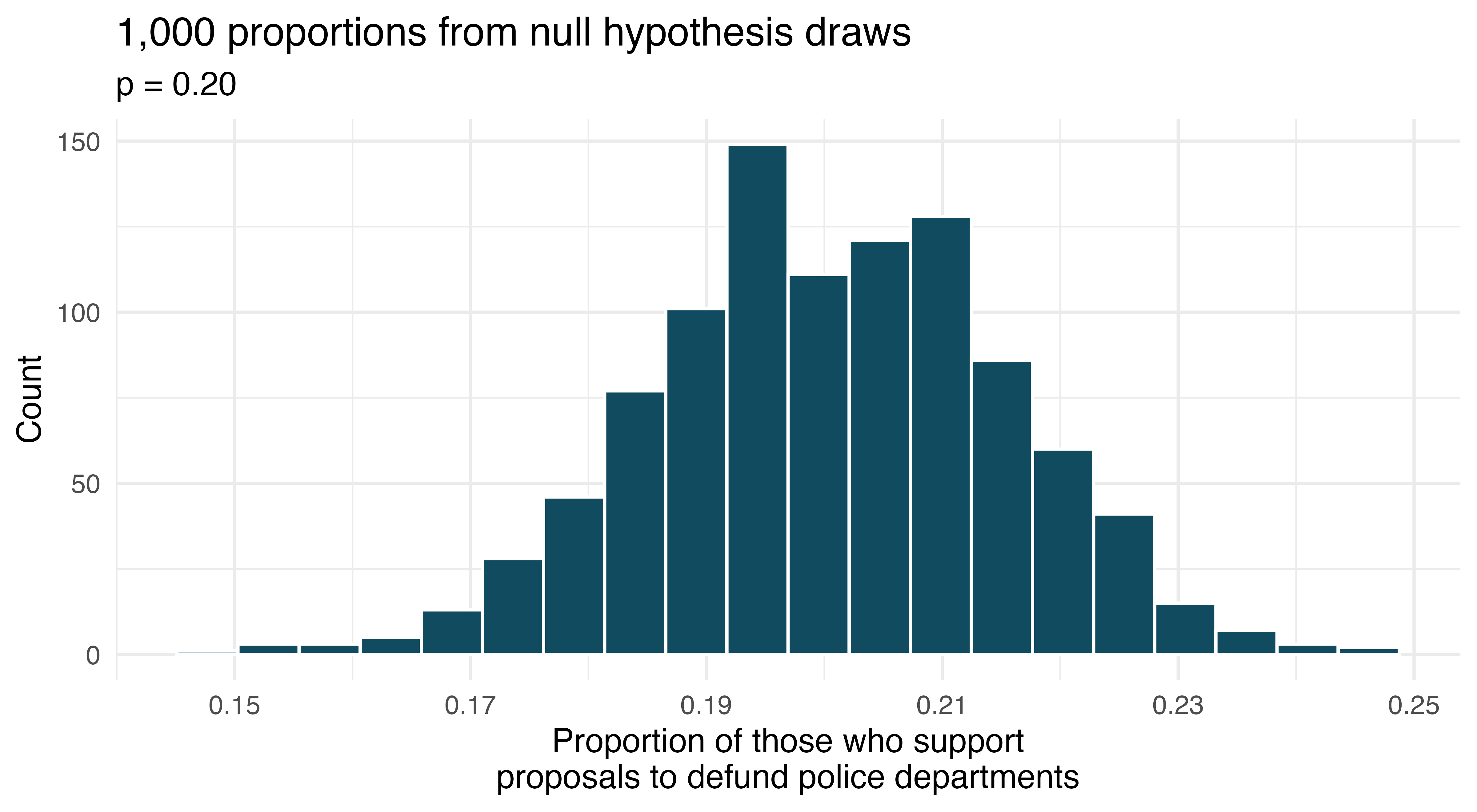
4. The histogram below shows the distribution of 1,000 $\hat{p}_{sim}$s under the null hypothesis. Estimate the p-value using the plot and use it to evaluate the hypotheses.

Assisted reproduction. Assisted Reproductive Technology (ART) is a collection of techniques that help facilitate pregnancy (e.g., in vitro fertilization). The 2018 ART Fertility Clinic Success Rates Report published by the Centers for Disease Control and Prevention reports that ART has been successful in leading to a live birth in 48.8% of cases where the patient is under 35 years old. (CDC 2018) A new fertility clinic claims that their success rate is higher than average for this age group. A random sample of 30 of their patients yielded a success rate of 60%. A consumer watchdog group would like to determine if the data provides strong evidence to support the company’s claim.
1. Write the hypotheses to test if the success rate for ART at this clinic is discernibly higher than the success rate reported by the CDC.
2. Describe a setup for a simulation that would be appropriate in this situation and how the p-value can be calculated using the simulation results.
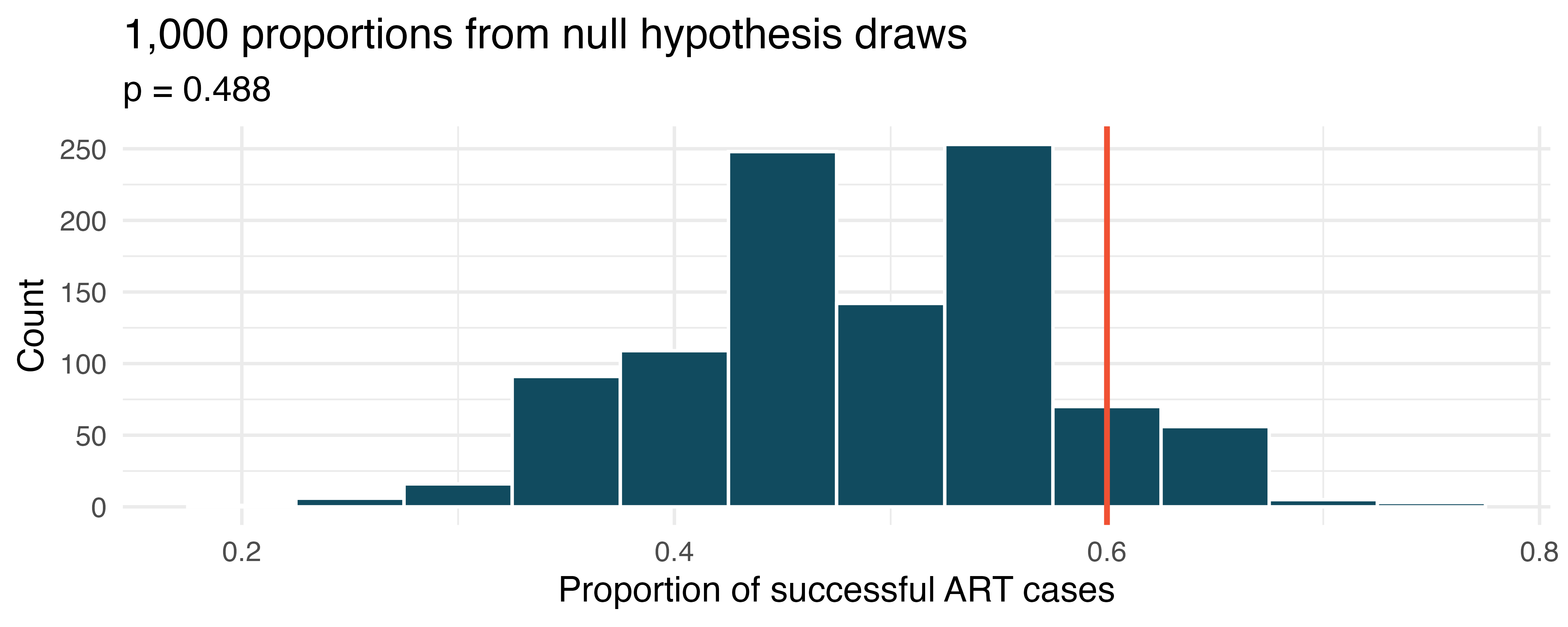
3. The histogram below shows the distribution of 1,000 $\hat{p}_{sim}$s under the null hypothesis. Estimate the p-value using the plot and use it to evaluate the hypotheses.
1. After performing this analysis, the consumer group releases the following news headline: “Infertility clinic falsely advertises better success rates”. Comment on the appropriateness of this statement.

If I fits, I sits, simulated null hypothesis. A citizen science project on which type of enclosed spaces cats are most likely to sit in compared (among other options) two different spaces taped to the ground. The first was a square, and the second was a shape known as Kanizsa square illusion. When comparing the two options given to 7 cats, 5 chose the square, and 2 chose the Kanizsa square illusion. We are interested to know whether these data provide convincing evidence that cats prefer one of the shapes over the other. (Smith et al. 2021)
1. What are the null and alternative hypotheses for evaluating whether these data provide convincing evidence that cats have preference for one of the shapes
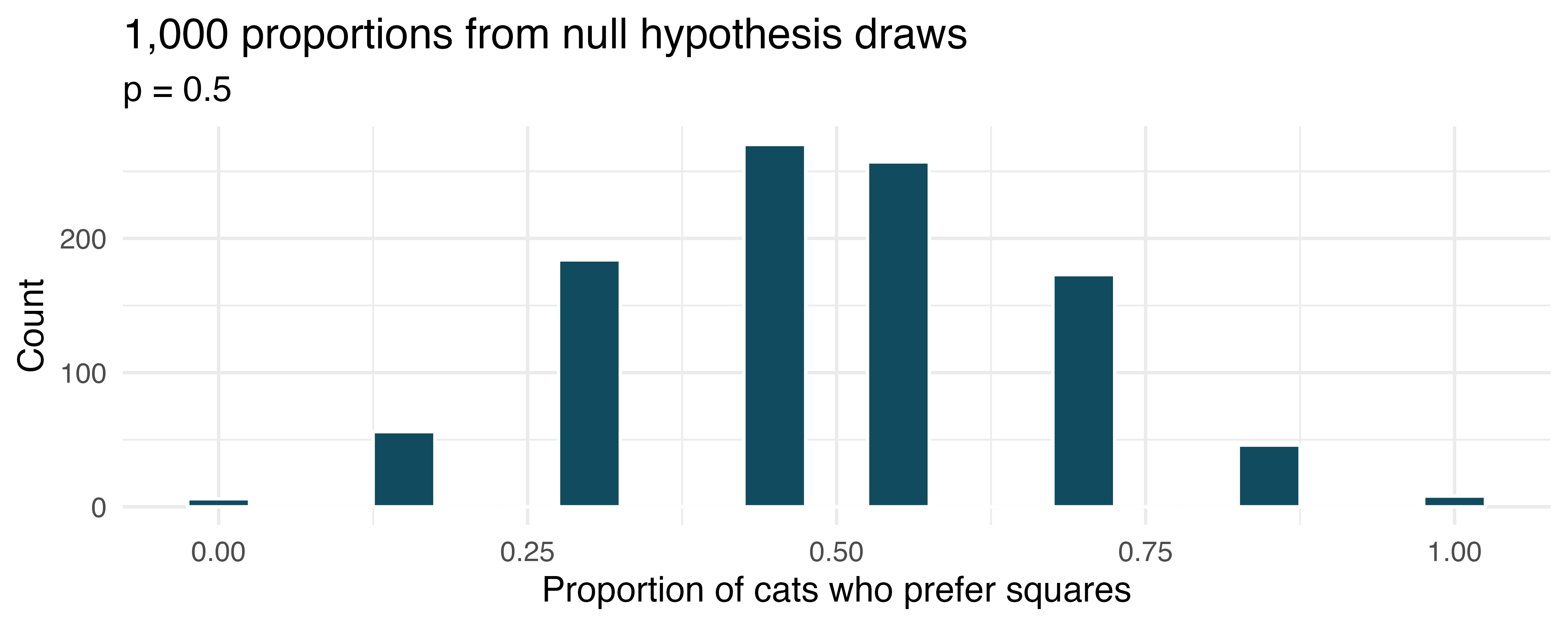
2. A null hypothesis simulation (with 1,000 draws) was run, and the resulting null distribution is displayed in the histogram below. Find the p-value using this distribution and conclude the hypothesis test in the context of the problem.

Legalization of marijuana, simulated null hypothesis. The 2022 General Social Survey asked a random sample of 1,207 US adults: “Do you think the use of marijuana should be made legal, or not?” 65.3% of the respondents said it should be made legal. (NORC 2022) Consider a scenario where, in order to become legal, 55% (or more) of voters must approve.
1. What are the null and alternative hypotheses for evaluating whether these data provide convincing evidence that, if voted on, marijuana would be legalized in the US.
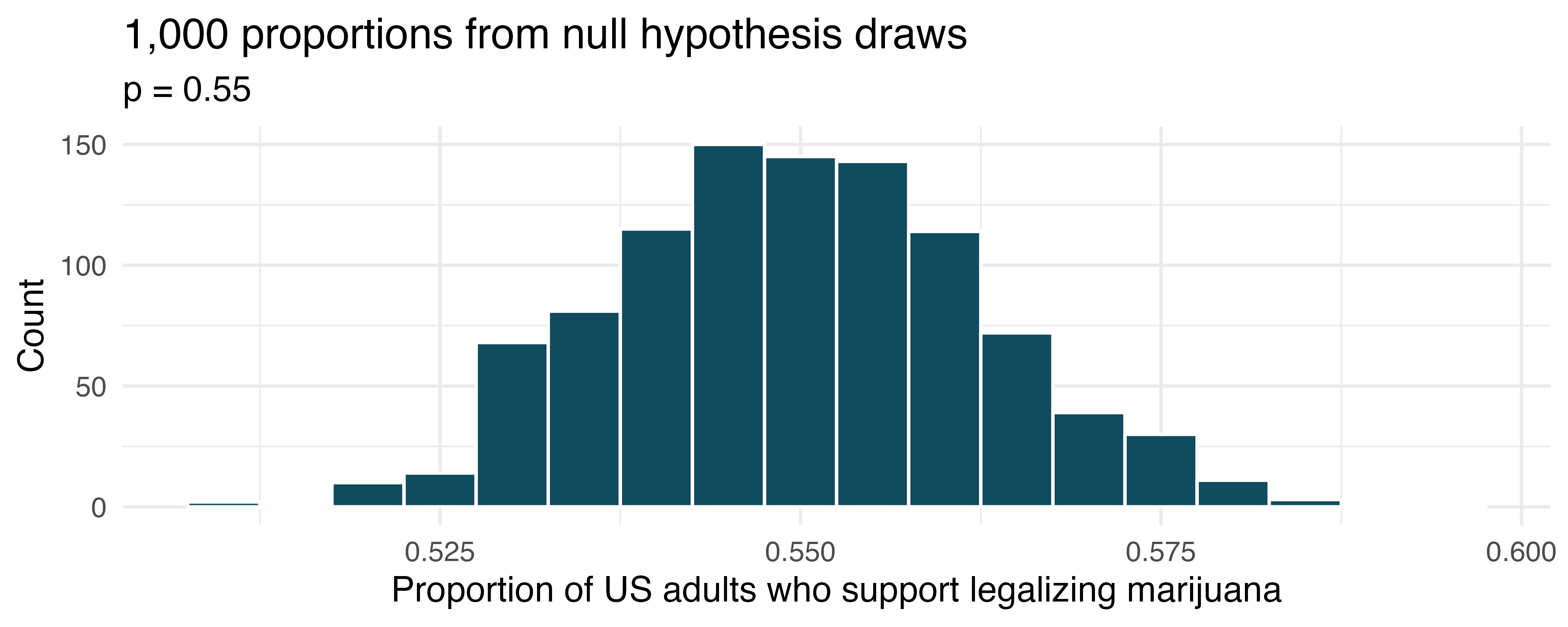
2. A null hypothesis simulation (with 1,000 draws) was run, and the resulting null distribution is displayed in the histogram below. Find the p-value using this distribution and conclude the hypothesis test in the context of the problem.

If I fits, I sits, standard errors. The results of a study on the type of enclosed spaces cats are most likely to sit in show that 5 out of 7 cats chose a square taped to the ground over a shape known as Kanizsa square illusion, which was preferred by the remaining 2 cats. To evaluate whether these data provide convincing evidence that cats prefer one of the shapes over the other, we set $H_0: p = 0.5$, where $p$ is the population proportion of cats who prefer square over the Kanizsa square illusion and $H_A: p \neq 0.5$, which suggests some preference, without specifying which shape is more preferred. (Smith et al. 2021)
1. Using the mathematical model, calculate the standard error of the sample proportion in repeated samples of size 7.
2. A null hypothesis simulation (with 1,000 draws) was run, and the resulting null distribution is displayed in the histogram below. This distribution shows the variability of the sample proportion in samples of size 7 when 50% of cats prefer the square shape over the Kanizsa square illusion. What is the approximate standard error of the sample proportion based on this distribution?
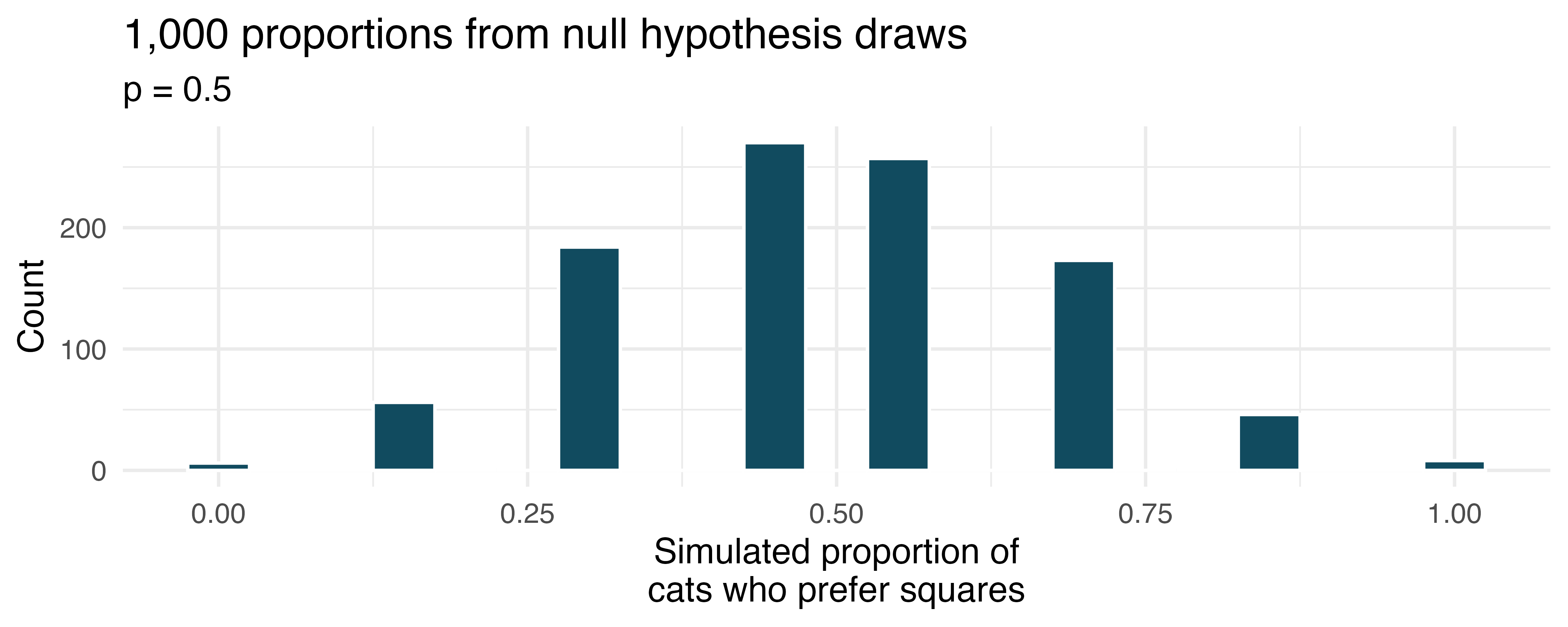
1. Do the mathematical model and simulated draws yield similar standard errors?
2. In order to approach the problem using the mathematical model, is the success-failure condition met for this study? Explain.
3. What features of the null distribution shown above tells us that the mathematical model should probably not be used?

Legalization of marijuana, standard errors. According to the 2022 General Social Survey, in a random sample of 1,207 US adults, 65.3% think marijuana should be made legal. (NORC 2022) Consider a scenario where, in order to become legal, 55% (or more) of voters must approve.
1. Calculate the standard error of the sample proportion using the mathematical model.
2. 1,000 sample proportions from samples of size 1,207 were drawn from a null distribution where 55% of voters approve legalizing marijuana. The distribution of these proportions is shown in the histogram below. Approximate the standard error of the sample proportion based on this distribution.
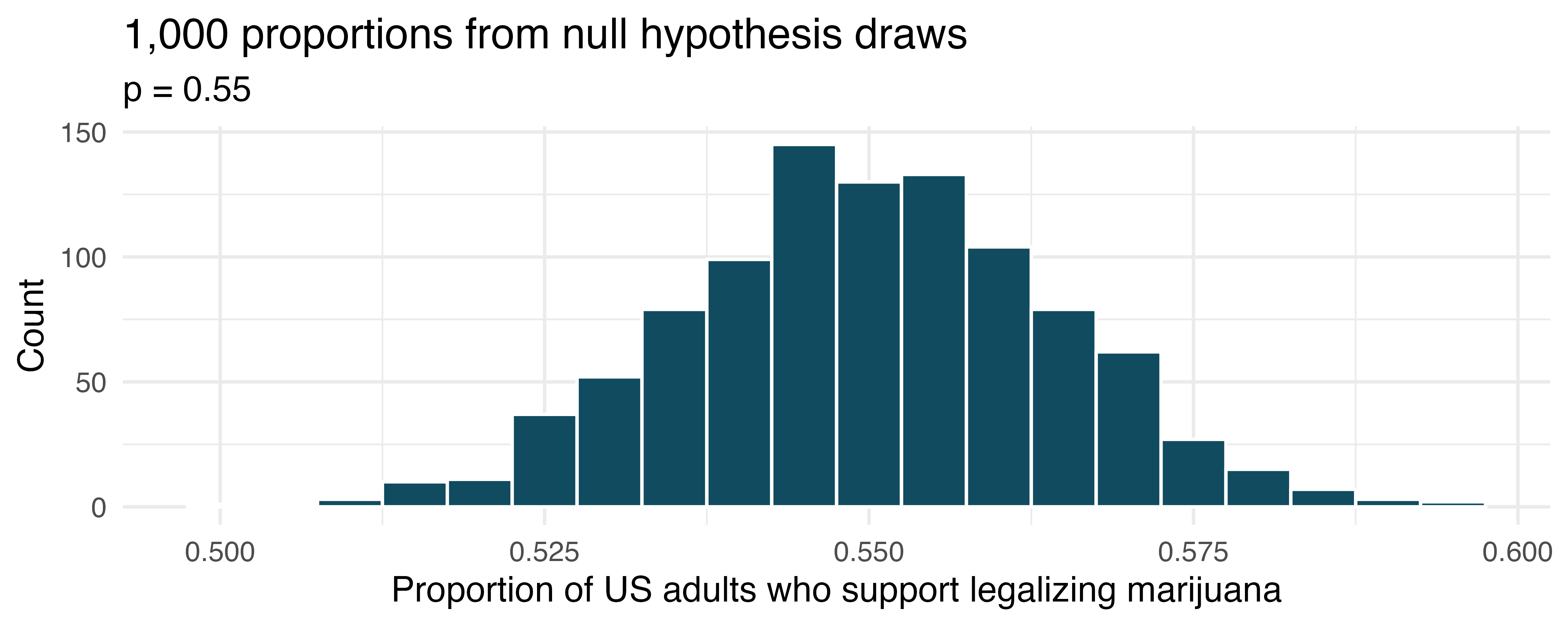
1. Do the mathematical model and simulated draws yield similar standard errors?
2. In this setting (to test whether the true underlying population proportion is greater than 0.55), would there be a strong reason to choose the mathematical model over the simulated null hypothesis (or vice versa)?

Statistics and employment, describe the bootstrap. A large university knows that about 70% of the full-time students are employed at least 5 hours per week. The members of the Statistics Department wonder if the same proportion of their students work at least 5 hours per week. They randomly sample 25 majors and find that 15 of the students work 5 or more hours each week.

Two sampling distributions are created to describe the variability in the proportion of statistics majors who work at least 5 hours per week. The null hypothesis simulation imposes a true population proportion of $p = 0.7$ while the data bootstrap resamples from the actual data (which has 60% of the observations who work at least 5 hours per week).
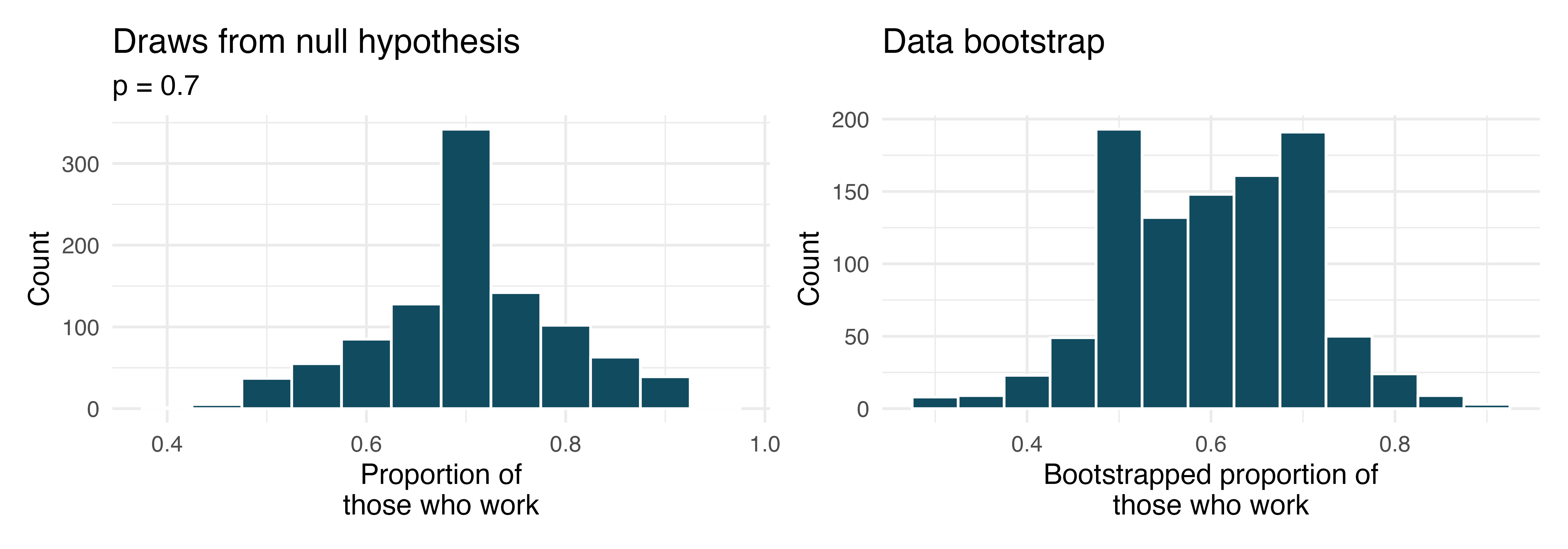
1. The sampling was done under two different settings to generate each of the distributions shown above. Describe the two different settings.
2. Where are each of the two distributions centered? How do their centers compare?
3. Estimate the standard error of the simulated proportions based on each distribution. Are the two standard errors you estimate roughly equal?
4. Describe the shapes of the two distributions. Are they roughly the same?

National Health Plan, simulated null hypothesis. A Kaiser Family Foundation poll for a random sample of US adults in 2019 found that 79% of Democrats, 55% of Independents, and 24% of Republicans supported a generic “National Health Plan”. There were 347 Democrats, 298 Republicans, and 617 Independents surveyed. (Kaiser Family Foundation 2019)

A political pundit on TV claims that a majority of Independents support a National Health Plan. Do these data provide strong evidence to support this type of statement? One approach to assessing the question of whether a majority of Independents support a National Health Plan is to simulate 1,000 draws from a null hypothesis with $p = 0.5$ as the proportion of Independents in support.
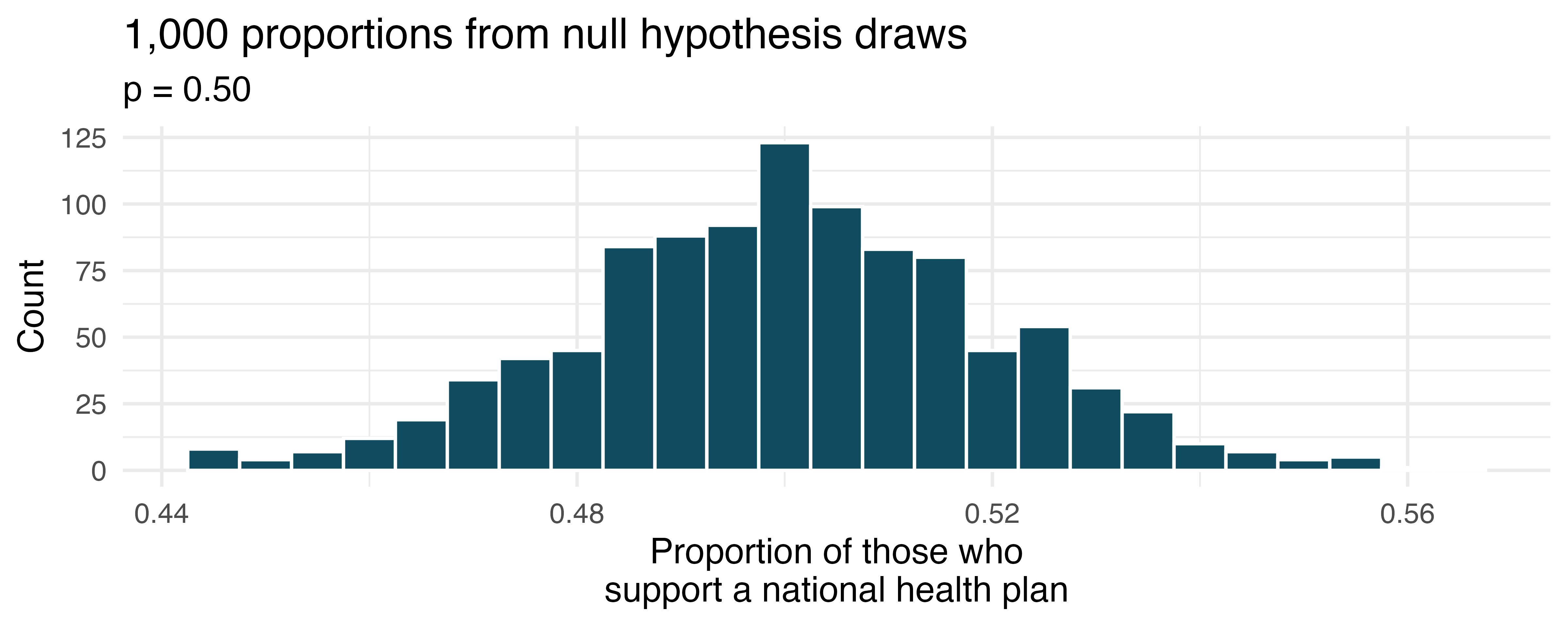
1. The histogram above displays 1000 values of what?
2. Is the observed proportion of Independents consistent with the null hypothesis simulated proportions under the setting where $p=0.5?$
3. In order to test the claim that “a majority of Independents support a National Health Plan” what are the null and alternative hypotheses?
4. Using the simulated null hypothesis distribution, find the p-value and conclude the hypothesis test in the context of the problem.
Statistics and employment, use the bootstrap. In a large university where 70% of the full-time students are employed at least 5 hours per week, the members of the Statistics Department wonder if the same proportion of their students work at least 5 hours per week. They randomly sample 25 majors and find that 15 of the students work 5 or more hours each week.

Two sampling distributions are created to describe the variability in the proportion of statistics majors who work at least 5 hours per week. The null hypothesis distribution imposes a true population proportion of $p=0.7$ while the data bootstrap resamples from the actual data (which has 60% of the observations who work at least 5 hours per week).
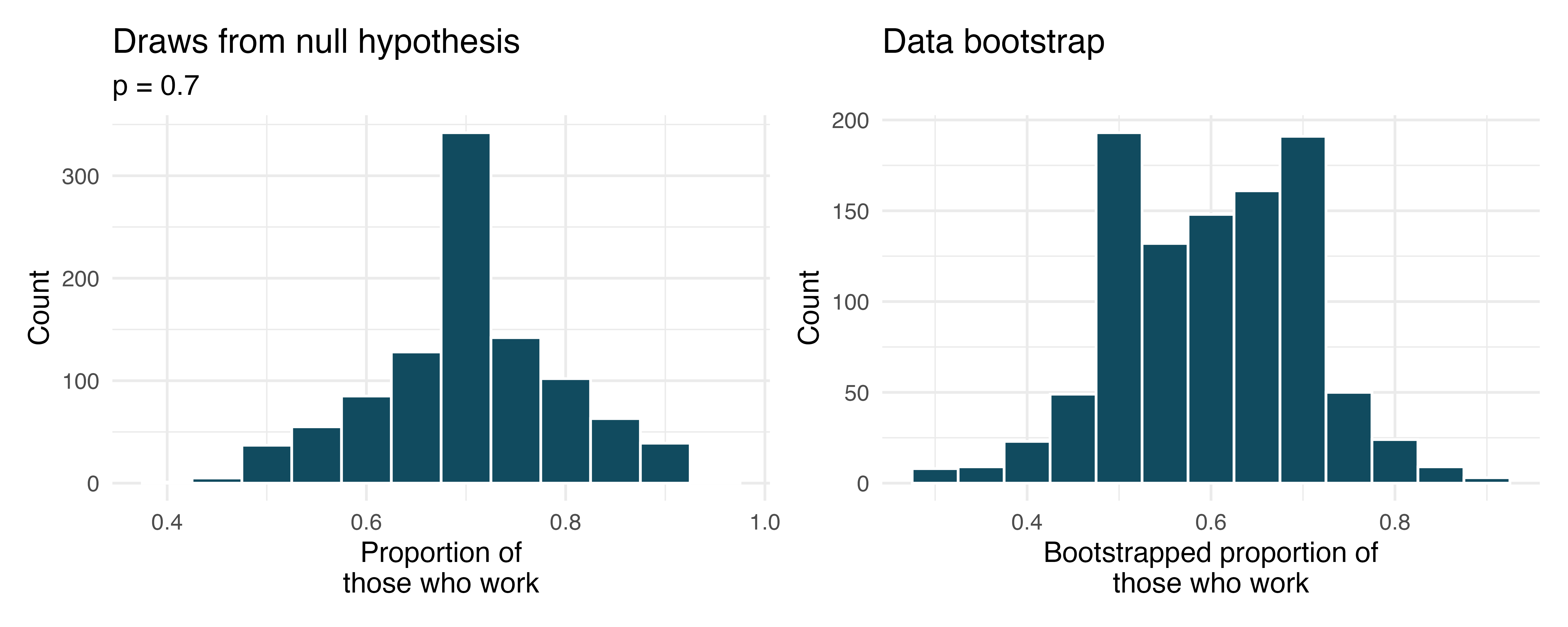
1. Which distribution should be used to test whether the proportion of all statistics majors who work at least 5 hours per week is 70%? And which distribution should be used to find a confidence interval for the true poportion of statistics majors who work at least 5 hours per week?
2. Using the appropriate histogram, test the claim that 70% of statistics majors, like their peers, work at least 5 hours per week. State the null and alternative hypotheses, find the p-value, and conclude the test in the context of the problem.
3. Using the appropriate histogram, find a 98% bootstrap percentile confidence interval for the true proportion of statistics majors who work at least 5 hours per week. Interpret the confidence interval in the context of the problem.
4. Using the appropriate historgram, find a 98% bootstrap SE confidence interval for the true proportion of statistics majors who work at least 5 hours per week. Interpret the confidence interval in the context of the problem.

CLT for proportions. Define the term “sampling distribution” of the sample proportion, and describe how the shape, center, and spread of the sampling distribution change as the sample size increases when $p = 0.1$.

Vegetarian college students. Suppose that 8% of college students are vegetarians. Determine if the following statements are true or false, and explain your reasoning.
1. The distribution of the sample proportions of vegetarians in random samples of size 60 is approximately normal since $n \ge 30$.
2. The distribution of the sample proportions of vegetarian college students in random samples of size 50 is right skewed.
3. A random sample of 125 college students where 12% are vegetarians would be considered unusual.
4. A random sample of 250 college students where 12% are vegetarians would be considered unusual.
5. The standard error would be reduced by one-half if we increased the sample size from 125 to 250.

Young Americans, American dream. About 77% of young adults think they can achieve the American dream. Determine if the following statements are true or false, and explain your reasoning. (Vaughn 2011)
1. The distribution of sample proportions of young Americans who think they can achieve the American dream in random samples of size 20 is left skewed.
2. The distribution of sample proportions of young Americans who think they can achieve the American dream in random samples of size 40 is approximately normal since $n \ge 30$.
3. A random sample of 60 young Americans where 85% think they can achieve the American dream would be considered unusual.
4. A random sample of 120 young Americans where 85% think they can achieve the American dream would be considered unusual.

Orange tabbies. Suppose that 90% of orange tabby cats are male. Determine if the following statements are true or false, and explain your reasoning.
1. The distribution of sample proportions of random samples of size 30 is left skewed.
2. Using a sample size that is 4 times as large will reduce the standard error of the sample proportion by one-half.
3. The distribution of sample proportions of random samples of size 140 is approximately normal.
4. The distribution of sample proportions of random samples of size 280 is approximately normal.

Young Americans, starting a family. About 25% of young Americans have delayed starting a family due to the continued economic slump. Determine if the following statements are true or false, and explain your reasoning. (Demos 2011)
1. The distribution of sample proportions of young Americans who have delayed starting a family due to the continued economic slump in random samples of size 12 is right skewed.
2. In order for the distribution of sample proportions of young Americans who have delayed starting a family due to the continued economic slump to be approximately normal, we need random samples where the sample size is at least 40.
3. A random sample of 50 young Americans where 20% have delayed starting a family due to the continued economic slump would be considered unusual.
4. A random sample of 150 young Americans where 20% have delayed starting a family due to the continued economic slump would be considered unusual.
5. Tripling the sample size will reduce the standard error of the sample proportion by one-third.

Sex equality. The General Social Survey asked a random sample of 1,390 Americans the following question: “On the whole, do you think it should or should not be the government’s responsibility to promote equality between men and women?” 82% of the respondents said it “should be”. At a 95% confidence level, this sample has 2% margin of error. Based on this information, determine if the following statements are true or false, and explain your reasoning. (NORC 2016)
1. We are 95% confident that 80% to 84% of Americans in this sample think it’s the government’s responsibility to promote equality between men and women.
2. We are 95% confident that 80% to 84% of all Americans think it’s the government’s responsibility to promote equality between men and women.
3. If we considered many random samples of 1,390 Americans, and we calculated 95% confidence intervals for each, 95% of these intervals would include the true population proportion of Americans who think it’s the government’s responsibility to promote equality between men and women.
4. In order to decrease the margin of error to 1%, we would need to quadruple (multiply by 4) the sample size.
5. Based on this confidence interval, there is sufficient evidence to conclude that a majority of Americans think it’s the government’s responsibility to promote equality between men and women.

Elderly drivers. A Marist Poll report states that 66% of American adults think licensed drivers should be required to retake their road test once they reach 65 years of age, based on a random sample of 1,018 American adults. They also report a margin of error was 3% at the 95% confidence level. (Poll 2011)
1. Verify the margin of error reported by The Marist Poll using a mathematical model.
2. Based on a 95% confidence interval, does the poll provide convincing evidence that more than two thirds of the population think that licensed drivers should be required to retake their road test once they turn 65?

Fireworks on July 4$^{\text{th}}$. A local news outlet reported that 56% of 600 randomly sampled Kansas residents planned to set off fireworks on July $4^{th}$. Determine the margin of error for the 56% point estimate using a 95% confidence level using a mathematical model. (Survey USA 2012)

Proof of COVID-19 vaccination. In the US, businesses and schools shut down due to the COVID-19 pandemic in March 2020, and a vaccine became publicly available for the first time in April 2021. That month, a Gallup poll surveyed a random sample of 3,731 US adults, asking how they felt about the COVID-19 vaccine requirement for air travel. The poll found that 57% said they would favor it. (Gallup 2021)
1. Describe the population parameter of interest. What is the value of the point estimate of this parameter?
2. Check if the conditions required for constructing a confidence interval using a mathematical model based on these data are met.
3. Construct a 95% confidence interval for the proportion of US adults who favor requiring proof of COVID-19 vaccination for travel by airplane.
4. Without doing any calculations, describe what would happen to the confidence interval if we decided to use a higher confidence level.
5. Without doing any calculations, describe what would happen to the confidence interval if we used a larger sample.

Study abroad. A survey on 1,509 high school seniors who took the SAT and who completed an optional web survey shows that 55% of high school seniors are fairly certain that they will participate in a study abroad program in college. (American Council on Education 2008)
1. Is this sample a representative sample from the population of all high school seniors in the US? Explain your reasoning.
2. Suppose the conditions for inference are met, regardless of your answer to part (a). Using a mathematical model, construct a 90% confidence interval for the proportion of high school seniors (of those who took the SAT) who are fairly certain they will participate in a study abroad program in college, and interpret this interval in context.
3. What does “90% confidence” mean?
4. Based on this interval, would it be appropriate to claim that the majority of high school seniors are fairly certain that they will participate in a study abroad program in college?

Legalization of marijuana, mathematical interval. The General Social Survey asked a random sample of 1,563 US adults: “Do you think the use of marijuana should be made legal, or not?” 60% of the respondents said it should be made legal. (NORC 2022)
1. Is 60% a sample statistic or a population parameter? Explain.
2. Using a mathematical model, construct a 95% confidence interval for the proportion of US adults who think marijuana should be made legal, and interpret it in the context of the data.
3. A critic points out that this 95% confidence interval is only accurate if the statistic follows a normal distribution, or if the normal model is a good approximation. Do the technical conditions hold for these data? Explain.
4. A news piece on this survey’s findings states, “Majority of US adults think marijuana should be legalized.” Based on your confidence interval, is the news piece’s statement justified?

National Health Plan, mathematical inference. A Kaiser Family Foundation poll for a random sample of US adults in 2019 found that 79% of Democrats, 55% of Independents, and 24% of Republicans supported a generic “National Health Plan”. There were 347 Democrats, 298 Republicans, and 617 Independents surveyed. (Kaiser Family Foundation 2019)
1. A political pundit on TV claims that a majority of Independents support a National Health Plan. Do these data provide strong evidence to support this type of statement? Your response should use a mathematical model.
2. Would you expect a confidence interval for the proportion of Independents who oppose the public option plan to include 0.5? Explain.

Is college worth it? Among a simple random sample of 331 American adults who do not have a four-year college degree and are not currently enrolled in school, 48% said they decided not to go to college because they could not afford school. (Pew Research Center 2011)
1. A newspaper article states that only a minority of the Americans who decide not to go to college do so because they cannot afford it and uses the point estimate from this survey as evidence. Conduct a hypothesis test to determine if these data provide strong evidence supporting this statement.
2. Would you expect a confidence interval for the proportion of American adults who decide not to go to college because they cannot afford it to include 0.5? Explain.

Taste test. Some people claim that they can tell the difference between a diet soda and a regular soda in the first sip. A researcher wanting to test this claim randomly sampled 80 such people. He then filled 80 plain white cups with soda, half diet and half regular through random assignment, and asked each person to take one sip from their cup and identify the soda as diet or regular. 53 participants correctly identified the soda.
1. Do these data provide strong evidence that these people are able to detect the difference between diet and regular soda, in other words, are the results discernibly better than just random guessing? Your response should use a mathematical model.
2. Interpret the p-value in this context.

Will the coronavirus bring the world closer together? In early 2020 the COVID-19 pandemic arrived in the US; by December 2020 the first COVID-19 vaccine was available. An April 2021 YouGov poll asked 4,265 UK adults whether they think the coronavirus bring the world closer together or leave us further apart. 12% of the respondents said it will bring the world closer together. 37% said it would leave us further apart, 39% said it won’t make a difference and the remainder didn’t have an opinion on the matter. (YouGov 2021)
1. Calculate, using a mathematical model, a 90% confidence interval for the proportion of UK adults who think the coronavirus will bring the world closer together, and interpret the interval in context.
2. Suppose we wanted the margin of error for the 90% confidence level to be about 0.5%. How large of a sample size would you recommend for the poll?

Quality control. As part of a quality control process for computer chips, an engineer at a factory randomly samples 212 chips during a week of production to test the current rate of chips with severe defects. She finds that 27 of the chips are defective.
1. What population is under consideration in the dataset?
2. What parameter is being estimated?
3. What is the point estimate for the parameter?
4. What is the name of the statistic that can be used to measure the uncertainty of the point estimate?
5. Compute the value of the statistic from part (d) using a mathematical model.
6. The historical rate of defects is 10%. Should the engineer be surprised by the observed rate of defects during the current week?
7. Suppose the true population value was found to be 10%. If we use this proportion to recompute the value in part (d) using $p = 0.1$ instead of $\hat{p}$, how much does the resulting value of the statistic change?

Nearsighted children. Nearsightedness (myopia) is a common vision condition in which you can see near objects clearly, but farther away objects blurry. It is believed that nearsightedness affects about 8% of all children. In a random sample of 194 children, 21 are nearsighted. Using a mathematical model, conduct a hypothesis test for the following question: do these data provide evidence that the 8% value is inaccurate?

Website registration. A website is trying to increase registration for first-time visitors, exposing 1% of these visitors to a new site design. Of 752 randomly sampled visitors over a month who saw the new design, 64 registered.
1. Check the conditions for constructing a confidence interval for the proportion of first-time visitors of the site who would register under the new design using a mathematical model.
2. Compute the standard error which would describe the variability os the point estimate associated with repeated samples of size 752.
3. Construct and interpret a 90% confidence interval for the fraction of first-time visitors of the site who would register under the new design (assuming stable behaviors by new visitors over time).

Coupons driving visits. A store randomly samples 603 shoppers over the course of a year and finds that 142 of them made their visit because of a coupon they’d received in the mail. Using a mathematical model, construct a 95% confidence interval for the fraction of all shoppers during the year whose visit was because of a coupon they’d received in the mail.

$H_0:$ There is no association between the consultant’s contributions and the clients’ complication rate. In statistical language, $p = 0.10.$ $H_A:$ Patients who work with the consultant tend to have a complication rate lower than 10%, i.e., $p < 0.10.$↩︎
There is not enough evidence to reject the null hypothesis in favor of the alternative hypothesis. We cannot conclude that there is evidence that the consultant’s surgery complication rate is lower than the US standard rate of 10%. That said, we also cannot conclude that there is evidence that the consultant’s surgery complication rate is higher than the US standard rate of 10%. When the p-value is larger than the discernibility level, we are unable to make conclusions about the research statement.↩︎
Not necessarily. There is no evidence to make a claim in either direction, so we cannot make any claims about whether the consultant is good at their job.↩︎
Because the $p$ is unknown but expected to be around 2/3, we will use 2/3 in place of $p$ in the formula for the standard error. $SE = \sqrt{\frac{p(1-p)}{n}} \approx \sqrt{\frac{2/3 (1 - 2/3)} {300}} = 0.027.$↩︎
This is equivalent to asking how often the $Z$ score will be larger than -2.58 but less than 2.58. (For a picture, see Figure 16.2.) To determine this probability, look up -2.58 and 2.58 in the normal probability table (0.0049 and 0.9951). Thus, there is a $0.9951-0.0049 \approx 0.99$ probability that the unobserved random variable $X$ will be within 2.58 standard deviations of the mean.↩︎
Since the necessary conditions for applying the normal model have already been checked for us, we can go straight to the construction of the confidence interval: $\text{point estimate} \pm 2.58 \times SE$ Which gives an interval of (0.018, 0.162).$ We are 99% confident that implanting a stent in the brain of a patient who is at risk of stroke increases the risk of stroke within 30 days by a rate of 0.018 to 0.162 (assuming the patients are representative of the population).↩︎
We must find $z^{\star}$ such that 90% of the distribution falls between -$z^{\star}$ and $z^{\star}$ in the standard normal model, $N(\mu=0, \sigma=1).$ We can look up -$z^{\star}$ in the normal probability table by looking for a lower tail of 5% (the other 5% is in the upper tail), thus $z^{\star} = 1.65.$ The 90% confidence interval can then be computed as $\text{point estimate} \pm 1.65 \times SE \to (4.4\%, 13.6\%).$ (Note: the conditions for normality had earlier been confirmed for us.) That is, we are 90% confident that implanting a stent in a stroke patient’s brain increased the risk of stroke within 30 days by 4.4% to 13.6%.
Note, the problem was set up as 90% to indicate that there was not a need for a high level of confidence (such as 95% or 99%). A lower degree of confidence increases potential for error, but it also produces a more narrow interval.↩︎
$H_0:$ there is not support for the regulation; $H_0:$ $p \leq 0.50.$ $H_A:$ the majority of borrowers support the regulation; $H_A:$ $p > 0.50.$↩︎
Independence holds since the poll is based on a random sample. The success-failure condition also holds, which is checked using the null value $(p_0 = 0.5)$ from $H_0:$ $np_0 = 826 \times 0.5 = 413,$ $n(1 - p_0) = 826 \times 0.5 = 413.$ Recall that here, the best guess for $p$ is $p_0$ which comes from the null hypothesis (because we assume the null hypothesis is true when performing the testing procedure steps). $H_0:$ there is not support for the regulation; $H_0:$ $p \leq 0.50.$ $H_A:$ the majority of borrowers support the regulation; $H_A:$ $p > 0.50.$↩︎

中文

16 单比例的推断

现在聚焦于分类数据的统计推断，我们将重新审视来自第 11.

的假设检验的许多基础方面。第 11, 第 12和第 13中的三种方法进行分析：随机化检验、自助法和数学模型。

我们详细讨论的三种数据结构是：一个二元变量，用单一比例来概括；两个二元变量，用两个比例之差来概括；以及两个分类变量，用双向表来概括。在适当的情况下，每种数据结构都将使用来自

的三种方法进行分析。第 12在逐步深入推断思想的过程中，我们将接触统计推断中新的基础概念。例如，我们将讨论正态模型适用的条件；假设检验中的两种不同错误率；以及如何为置信区间选择置信水平。

我们在

16.1 中遇到过单一比例的推断方法，探讨了点估计和置信区间。在本节中，我们将复习这些主题，以及如何在收集单一比例情境的数据时选择合适的样本量。

请注意，在关注单一比例的研究中，只测量一个变量。对于每个观测单元，该单一变量被测量为成功或失败（例如，“手术并发症”与“无手术并发症”）。由于当前研究问题的性质只关注单一变量，因此无法将该变量跨另一个（解释性）变量进行随机化。因此，在关注单一比例时，我们不会使用随机化作为分析工具。相反，我们将应用Bootstrap技术来检验给定的假设，并且我们还将重新审视相关的数学模型。 $H_0$ 为真是类似于在第 12 中介绍的案例研究中所使用的思想，我们在那里进行自助法时不对 $H_0.$ 作任何假设。 $p$ 因为我们将要检验一个假设值 $p_0),$ （称为

），用于假设检验的自助法模拟有一个极好的优点：它可以用于任何样本量（对小样本是巨大的好处，对大样本则是一个不错的替代方法）。第 12.1 节我们扩展

16.1.1 观测数据

中的医疗顾问例子，但这次不是求真实并发症率的区间估计，而是检验一个具体的说法。

回顾该例子的背景：提供器官捐赠的人有时会寻求一种特殊“医疗顾问”的帮助。这些顾问在手术的各个方面协助患者，目标是在医疗过程和恢复期间减少出现并发症的可能性。患者可能会部分基于顾问客户的历史并发症率来选择顾问。一位顾问试图通过以下说法吸引患者：美国肝脏捐赠手术的平均并发症率约为10%，而在她经手的62例肝脏捐赠手术中，她的客户只出现了3例并发症。她声称这是强有力的证据，表明她的工作切实有助于减少并发症（因此应该雇用她！）。

利用这些数据，能否评估该顾问关于她的并发症率低于10%的说法？

不能。该说法是一个因果联系，但数据是观察性的。雇用这位医疗顾问的患者可能由于其他原因而有较低的并发症率。 $\hat{p} = 0.0484$ 虽然无法评估这一因果性说法，但仍可以用这些数据检验是否存在关联。对于这个问题我们要问：如果她的并发症率与美国标准率没有差别，那么

的低并发症率是否可能仅仅是偶然发生的？ $p,$ 用通俗语言和统计语言分别写出假设，以检验顾问的工作与真实并发症率¹

（针对顾问的客户）之间的关联。因为，事实证明，使用正态分布的条件并不满足（参见 Section 16.2)，与样本比例相关的不确定性不应使用正态分布来建模，因为这样做会低估与样本统计量相关的不确定性。然而，在没有正态框架的情况下，我们仍然希望评估之前“引导练习”中的假设。为此，我们需要评估出现一个样本值的可能性，该样本值 $(\hat{p})$ 与观察到的值一样低于零假设值。样本值与假设参数之间的偏差通常用 p 值来量化。 $p_0 = 0.10$ p 值是基于零假设分布计算的，零假设分布是当零假设为真时检验统计量的分布。假设零假设为真，我们可以通过确定观察到至少与观察到的检验统计量一样强烈地支持备择假设的检验统计量的概率来计算 p 值。这里我们将使用自助法模拟来计算 p 值。

我们想要确定当零假设为真时检验统计量

16.1.2 统计量的变异性

的抽样分布。换句话说，我们想了解当零假设为真时，样本比例可能出现的变异性。然后我们计划利用这些信息来判断是否有足够的证据拒绝零假设。 $(\hat{p})$ 在零假设下，10% 的肝脏捐献者在手术期间或术后出现并发症。假设对于该顾问的客户（针对

该顾问的所有客户，而不仅仅是之前测量的 62 位），这一比例确实没有什么不同。如果是这样，我们可以所有模拟 62 位客户，从零假设分布中获得并发症率的样本比例。使用假设的零参数值进行观测模拟通常被称为 参数自助法模拟 ，但我们将描述性地称之为“在零假设主张下进行模拟”。与

与第 12 章所述过程类似，可以用一个装有 10% 红色弹珠和 90% 白色弹珠的袋子模拟每位客户。从袋中抽取一颗弹珠，是在真实并发症率为 10%的前提下模拟患者是否出现并发症的一种方式。如果抽取 62 颗弹珠，再计算模拟中出现并发症患者的比例 $\hat{p}_{sim1},$，所得样本比例就是从零分布中抽取的一个样本。

共有 5 个模拟病例出现并发症，57 个模拟病例未出现并发症，即， $\hat{p}_{sim1} = 5/62 = 0.081.$

仅凭这一次模拟是否足以确定我们是否应该拒绝原假设？

不能。为了评估这些假设，我们需要看到许多个 $\hat{p}_{sim},$ 值的分布， 而不仅仅是 从该抽样分布中抽取的一次结果。

16.1.3 观测统计量与零假设统计量的对比

一次模拟不足以了解零分布的情况；需要进行多次模拟研究。大约 10,000 次似乎就足够了。然而，花钱请人手工模拟 10,000 项研究是浪费时间和金钱。相反，模拟通常通过编程在计算机上进行，这样效率要高得多。

图 16.1 展示了 10,000 次模拟研究的结果。等于或小于 $\hat{p} = 0.0484$ 的比例被阴影标出。阴影区域代表零分布下提供的证据至少与 $\hat{p}$ 支持备择假设的证据相当的样本比例。共有 1170 个模拟样本比例满足 $\hat{p}_{sim} \leq 0.0484.$ 我们用这些来构造零分布的左尾区域并求出 p 值：

\[\text{left tail area} = \frac{\text{Number of observed simulations with }\hat{p}_{sim} \leq \text{ 0.0484}}{10000}\]

在 10,000 个模拟的 $\hat{p}_{sim},$ 中，有 1170 个等于或小于 $\hat{p}.$ 。由于该假设检验是单侧的，估计的 p 值就等于这个尾部的面积：0.117。

由于估计的 p 值为 0.117，大于可辨别水平 0.05，我们不能拒绝原假设。请用通俗的语言解释这在问题背景下意味着什么。²

前一个引导练习中的结论是否意味着这位顾问擅长他们的工作？请解释。³

的零分布 $\hat{p}$ （使用自助法模拟）。

无论选择哪种统计方法，p 值总是通过分析检验统计量的零分布得出的。当成功-失败条件不满足时，正态模型对 $\hat{p}$ （样本比例）的零分布近似效果很差。作为替代，我们可以通过模拟样本比例来生成零分布，并利用该分布计算尾面积，即 p 值。

在前一个引导练习中，p 值是 估计的。它不是精确值，因为模拟的零分布本身只是样本统计量抽样分布的近似。可以使用二项分布生成精确的 p 值，但该方法不在本书的讨论范围内。

16.2 比例的数学模型

16.2.1 条件

在第 13.2 节中，我们介绍了正态分布，并展示了如何将其用作描述统计量变异性的数学模型。在某些条件下，样本比例 $\hat{p}$ 可以很好地用正态分布建模。当观测值相互独立且样本量足够大时，正态模型能相当好地描述样本比例的抽样分布；当观测值违反这些条件时，正态模型可能不准确，尤其可能低估样本比例的变异性。

的抽样分布 $\hat{p}.$

基于样本量 $\hat{p}$ 、来自真实比例为 $n$ 的总体的样本， $p$ 在以下条件下近似正态：

样本的观测值相互独立，例如来自简单随机样本。
我们预期样本中至少有 10 次成功和 10 次失败，即 $np\geq10$ 和 $n(1-p)\geq10.$ 这被称为 成功-失败条件.

当这些条件满足时， $\hat{p}$ 的抽样分布近似正态，均值为 $p$ ，标准误为 $\hat{p}$ 因为 $SE = \sqrt{\frac{\ \hat{p}(1-\hat{p})\ }{n}}.$

回忆一下，误差幅度由标准误差定义。 $\hat{p}$ 的误差幅度可以直接从 $SE(\hat{p}).$

误差幅度（针对 $\hat{p}.$

误差幅度为 $z^\star \times \sqrt{\frac{\ \hat{p}(1-\hat{p})\ }{n}}$ ，其中 $z^\star$ 是根据正态分布的某个指定百分位数计算得出的。

通常我们不知道真实比例 $p,$ ，因此我们用某个替代值来检验条件并估计标准误。对于置信区间，使用样本比例 $\hat{p}$ 来检验成功-失败条件并计算标准误。对于假设检验，通常使用零值——即零假设中声称的比例——来代替 $p.$

独立性条件是一个更为微妙的要求。当该条件不满足时，重要的是理解它是如何以及为何被违反的。例如，对于来自方便样本的数据，目前没有任何统计方法能够真正纠正其固有的偏差。另一方面，如果我们采用整群抽样（参见第 2.1.5 节），观测值将不是独立的，但有合适的统计方法可用于分析这些数据（不过这些方法超出了大多数统计学第二或第三门课程的范围）。

在基于大样本理论的例子中，我们用正态分布对 $\hat{p}$ 进行了建模。为什么这不适用于医疗顾问的案例研究？

如果每台手术来自不同的手术团队，独立性假设可能是合理的。然而，成功-失败条件不满足。在原假设下，我们预计会看到 $62 \times 0.10 = 6.2$ 例并发症，而不是正态近似所需的 10 例。

虽然本书的范围限定在约束良好的统计问题上，但请记住，这只是庞大统计方法库中的第一本书，这些方法适用于非常广泛的数据和情境。

16.2.2 比例的置信区间

置信区间为参数 $p,$ 提供了一个合理取值范围，并且当 $\hat{p}$ 可以用正态分布建模时， $p$ 的置信区间具有如下形式 $\hat{p} \pm z^{\star} \times SE.$ 我们已经看到 $\hat{p}$ 是样本比例。数值 $z^{\star}$ 决定置信水平（之前设为 1.96），并将在后面的例子中详细讨论。标准误 $SE,$ 的值在很大程度上取决于样本量。

单个比例的标准误， $\hat{p}.$

当条件满足使得 $\widehat{p}$ （样本比例）的分布近似正态时， 变异性 单一比例的， $\widehat{p}$ 可以很好地由以下公式描述：

\[SE(\hat{p}) = \sqrt{\frac{p(1-p)}{n}}\]

请注意，我们几乎从来不知道 $p$ 的真实值（总体概率或比例）。一个更有用的公式是：

\[ SE(\hat{p}) \approx \sqrt{\frac{(\mbox{best guess of }p)(1 - \mbox{best guess of }p)}{n}} \]

对于假设检验，我们使用 $p_0$ （原假设中规定的比例）作为 $p.$ 的最佳猜测。对于置信区间，我们使用 $\widehat{p}$ 作为 $p.$

的最佳猜测。 $(\hat{p})$ 考虑对登记选民（即随机样本）进行多次规模为300的民意调查，询问他们是否支持大麻合法化。据推测，大约2/3的选民支持大麻合法化。为了了解样本比例 $\hat{p}.$⁴

16.2.3 样本比例的变异性

在各样本之间的变化情况，计算

的标准误。 $\hat{p}$ 为更好地了解发薪日贷款借款人对监管和成本的看法，对826名发薪日贷款借款人进行了简单随机抽样调查。70%的回复支持对发薪日贷款机构实施新规。
估计 $\hat{p}.$
使用正态分布对 $p,$ 的分布进行建模是否合理？

为发薪日贷款借款人中支持加强对发薪日贷款机构监管的比例构造一个95%的置信区间。由于数据是随机样本，因此可以合理地假设观测值是相互独立的，并且能够代表目标总体。我们还必须使用 $\hat{p}$ 代替 $p$ 在计算置信区间时。由于两个值都至少为 10，我们可以使用正态分布来建模 $\hat{p}.$

\[ \begin{aligned} \text{Support: } n p & \approx 826 \times 0.70 = 578\\ \text{Not: } n (1 - p) & \approx 826 \times (1 - 0.70) = 248 \end{aligned} \] 2. 因为 $p$ 未知，且标准误是用于置信区间的，所以在公式中使用 $\hat{p}$ 代替 $p$ 。

\[SE = \sqrt{\frac{p(1-p)}{n}} \approx \sqrt{\frac{0.70 (1 - 0.70)} {826}} = 0.016.\]

使用 $\hat{p} = 0.70$, $z^{\star} = 1.96$ 对于 95% 置信区间，以及来自上一个引导练习的标准误 $SE = 0.016$ ，置信区间为

\[ \begin{aligned} \text{point estimate} \ &\pm \ z^{\star} \times \ SE \\ 0.70 \ &\pm \ 1.96 \ \times \ 0.016 \\ (0.669 \ &, \ 0.731) \end{aligned} \] 我们有 95% 的信心认为，在民意调查时支持监管的发薪日贷款借款人的真实比例介于 0.669 和 0.731 之间。

构建单个比例的置信区间。

构建 $p$ （真实的总体比例或概率）的置信区间有三个步骤。

检查假设观测值相互独立是否合理，并使用 $\hat{p}$ （样本比例）检查成功-失败条件。如果条件满足，则 $\hat{p}$ 的抽样分布可以很好地用正态模型近似。
使用 $\hat{p}$ 而不是 $p$.
计算标准误。应用一般置信区间公式。

有关更多单比例置信区间的例子，请参见第 12.3 节.

16.2.4 改变置信水平

假设我们想考虑置信水平略高于 95% 的置信区间：比如我们想要 99% 的置信水平。回想一下捕鱼的比喻：如果我们想更有把握捕到鱼，就应该使用更宽的网。要创建 99% 的置信水平，我们也必须加宽我们的 95% 区间。另一方面，如果我们想要一个置信水平较低的区间，比如 90%，我们可以把原来的 95% 区间稍微收窄一些。

95% 置信区间的结构为如何构建具有新置信水平的区间提供了指导。下面是一个来自近似正态分布的点估计的一般 95% 置信区间：

\[ \text{point estimate} \ \pm \ 1.96 \ \times \ SE \]

这个区间有三个组成部分：点估计值、“1.96”和标准误。选择 $1.96 \times SE$ 的依据是要涵盖 95% 的数据，因为估计值大约有 95% 的时间位于真实值的 1.96 个标准误之内。1.96 对应于 95% 的置信水平。

如果 $X$ 是一个服从正态分布的随机变量，那么 $X$ 有多少概率会落在均值的 2.58 个标准差范围内？⁵

要创建 99% 的置信区间，将 95% 置信区间公式中的 1.96 改为 $2.58.$ 。前面的引导练习强调了正态随机变量有 99% 的时间会落在其均值的 2.58 个标准差范围内。这种方法——使用正态模型中的 Z 分数来计算置信水平——适用于点估计与正态分布相关联且我们能够正确计算标准误的情况。因此，99% 置信区间的公式为：

\[ \text{point estimate} \ \pm \ 2.58 \ \times \ SE \]

正态近似对 $z^\star$ 置信区间（与自助法百分位置信区间相对）。当正态模型拟合效果不佳时，我们将使用能更好刻画抽样分布的替代分布，或者使用自助法程序。

使用来自第1.1节的数据，为支架对中风风险的影响构建一个99%置信区间。点估计值为0.090，标准误为 $SE = 0.028.$ 。已经为你验证过，该点估计值可以合理地用正态分布来建模。⁶

任意置信水平下的数学模型置信区间。

如果点估计值服从标准误为 $SE,$ 的正态模型，则总体参数的置信区间为

\[ \text{point estimate} \ \pm \ z^{\star} \ \times \ SE \]

其中 $z^{\star}$ 对应于所选的置信水平。

图 16.2 展示了如何根据置信水平确定 $z^{\star}$ 。我们选取 $z^{\star}$ ，使得正态模型中 -$z^{\star}$ 和 $z^{\star}$ 之间的面积对应于该置信水平。

之前我们发现，对有中风风险的患者在脑部植入支架会增加中风的风险。该研究估计中风患者数量增加了9%，且该估计的标准误约为 $SE = 2.8%.$ 。计算该效应的90%置信区间。⁷

16.2.5 比例的假设检验

对发薪日贷款机构的一种可能监管是，要求它们进行信用检查，并根据借款人的财务状况评估其债务偿还能力。我们想知道：借款人是否会支持这种形式的监管？

建立假设，以评估借款人是否对这类监管有大多数支持。⁸

要在比例假设检验的情境中应用正态分布框架，必须满足独立性和成功-失败条件。在假设检验中，成功-失败条件使用原假设比例来检验：我们验证 $np_0$ 和 $n(1-p_0)$ 至少为 10，其中 $p_0$ 是原假设值。

评估单个比例的检验统计量是 Z。

该 Z分数 是一个比值，衡量样本比例与假设比例 $(p_0)$ 的差异，相对于 $\hat{p}$ （样本比例）值的预期变异性。

\[ Z = \frac{\hat{p} - p_0}{\sqrt{p_0(1 - p_0)/n}} \]

当原假设为真且条件满足时，Z 服从标准正态分布。

F 统计量是各组之间差异程度（MSG）与组内观测值变异程度（MSE）的比值。

独立观测
大样本 $(n p_0 \geq 10$ 和 $n (1-p_0) \geq 10)$

发薪日贷款借款人是否支持一项要求贷款机构调取其信用报告并评估其债务偿还情况的监管？在 826 名借款人的随机样本中，51% 表示他们会支持这样的监管。在这里的假设检验中，使用正态分布来建模 $\hat{p}$ 是否合理？⁹

比例假设检验的数学模型。

建立假设并使用原假设值验证条件， $p_0,$ 以确保 $\hat{p}$ （样本比例）在 $H_0.$ 下接近正态。如果这些条件成立，则计算标准误，同样使用 $p_0,$ ，并在图中标出 p 值。最后，计算 p 值并评估假设。

有关单比例假设检验的更多示例，请参见第 11.3 节.

利用之前的引导练习中设定的假设和数据，评估关于放贷规定的民意调查是否提供了令人信服的证据，表明大多数发薪日贷款借款人支持一项新规定，该规定要求放贷方调取信用报告并评估债务偿还情况。

假设已经设定且条件已检验，我们可以进行计算。单比例假设检验中的标准误使用原值 $p_0:$

\[ SE = \sqrt{\frac{p_0 (1 - p_0)}{n}} = \sqrt{\frac{0.5 (1 - 0.5)}{826}} = 0.017 \]

计算。

下方展示了正态模型的图像，p 值由阴影区域表示。

\[ Z = \frac{\text{point estimate} - \text{null value}}{SE} = \frac{0.51 - 0.50}{0.017} = 0.59 \]

基于正态模型，检验统计量可以计算为点估计的 Z 分数： $H_0.$ 表示 p 值的单侧尾部面积为 0.2776。由于 p 值大于 0.05，我们不拒绝

在。该民意调查并未提供令人信服的证据，表明大多数发薪日贷款借款人支持关于信用审查和债务偿还评估的规定。第 17.1 节 中，我们讨论了双侧假设检验，发薪日贷款的例子可能更适合采用这种结构。也就是说，我们可能想问借款人是 支持还是反对（或反对）这些规定（以研究偏离 50% 基准任一方向的舆论）。在这种情况下，p 值将加倍为 0.5552（同样，我们不会拒绝 $H_0).$ 在双侧假设检验的情境下，恰当的结论应该是：该民意调查并未提供令人信服的证据，表明大多数发薪日贷款借款人支持或反对有关信用审查和债务偿还评估的规定。

无论在单侧还是双侧检验的情境下，这个结论都有些不尽如人意，因为没有得出任何结论。也就是说，对于公众舆论没有得出任何倾向性的结果。我们不能断言恰好有50%的人支持该规定，但也不能断言任何一方占多数。

16.2.6 违反条件

我们已经花了大量时间讨论在什么条件下 $\hat{p}$ 可以用正态分布合理建模。那么当成功-失败条件不满足时会发生什么？当独立性条件不满足时又会怎样？无论哪种情况，置信区间和假设检验的基本思想保持不变，但用于生成区间或p值的策略或技术会有所不同。

当成功-失败条件在假设检验中不满足时，我们可以使用原假设值 $\hat{p}$ 来模拟 $p_0,$ 的原分布，如第 16.1 节所示。遗憾的是，处理非独立观测值的方法（例如，对研究对象进行研究中前后重复测量）超出了本书的范围。

16.3 本章复习

16.3.1 小结

在前几节基础思想的基础上，本章专门讨论了单一总体比例作为感兴趣的参数。请注意，仅有一个变量时无法进行随机化检验，因此为了进行计算假设检验，我们采用了自助法（bootstrapping）框架。自助置信区间以及用于假设检验和置信区间的数学框架与其他数据结构和参数所用的方法类似。使用数学模型时，请牢记成功-失败条件。此外，要知道自助法在样本量较大时总是更准确。

16.3.2 术语

本章中介绍的术语列于表 16.1。如果您不确定其中一些术语的含义，我们建议您回到正文中复习它们的定义。您应该能够很容易地发现它们是 粗体文本.

表 16.1：本章介绍的术语。

参数自助法	成功-失败条件
单一比例标准误	Z分数

16.4 练习

奇数编号习题的答案见附录 A.16.

外星人存在吗？ 2021年5月，YouGov询问了4,839名英国成年居民，他们是否认为外星人存在，如果存在，他们是否曾造访地球。你想评估是否超过四分之一（25%）的英国成年人认为外星人不存在。在调查中，22%的人回答“我认为外星人存在，并且曾造访地球”，28%的人回答“我认为外星人存在，但未曾造访地球”，29%的人回答“我认为外星人不存在”，22%的人回答“不知道”。你的一位朋友主动帮你建立假设检验，并提出了以下假设。请指出你发现的任何错误。

$H_0: \hat{p} = 0.29 \quad \quad H_A: \hat{p} > 0.29$

25岁结婚。 一项研究表明，25岁的年轻人中有25%已经结婚。你认为这是错误的，于是决定收集自己的样本进行假设检验。在776名25岁年轻人的随机样本中，你发现有24%的人已婚。你的一位朋友主动提出帮你建立假设检验，并提出了以下假设。请指出你发现的任何错误。

$H_0: \hat{p} = 0.24 \quad \quad H_A: \hat{p} \neq 0.24$

撤资警察。 2021年5月在华盛顿州西雅图进行的一项Survey USA民意调查显示，在650名受访者（居住在该地区的成年人）中，有159人支持削减警察部门经费的提案。 (Survey USA 2021)
1. 一位撰写有关该民调结果新闻报道的记者想使用标题“西雅图超过五分之一的成年人支持削减警察部门经费的提案”。你提醒记者，他们应该先进行假设检验，以查看民调数据是否为这一说法提供了令人信服的证据。请写出该检验的假设。
2. 计算样本中支持削减警察部门经费提案的西雅图成年人的比例。
3. 描述一种适用于这种情况的模拟设置，以及如何利用模拟结果计算p值。
4. 下面的直方图显示了1,000个 $\hat{p}_{sim}$零假设下的 s。利用图形估计 p 值，并用它来评估假设。

辅助生殖。 辅助生殖技术（ART）是一系列帮助促进怀孕的技术（例如体外受精）。美国疾病控制与预防中心发布的《2018年ART生育诊所成功率报告》指出，在患者年龄小于35岁的病例中，ART成功实现活产的比例为48.8%。 (CDC 2018) 一家新的生育诊所声称，他们在这个年龄组的成功率高于平均水平。对其30名患者的随机样本显示成功率为60%。一个消费者监督组织想确定这些数据是否提供了强有力的证据来支持该公司的说法。
1. 写出检验该诊所ART成功率是否明显高于CDC报告的成功率的假设。
2. 描述一种适用于这种情况的模拟设置，以及如何利用模拟结果计算p值。
3. 下面的直方图显示了1,000个 $\hat{p}_{sim}$零假设下的 s。利用图形估计 p 值，并用它来评估假设。
1. 完成这一分析后，消费者团体发布了以下新闻标题：“不孕不育诊所虚假宣传更高的成功率”。请评论这一说法是否恰当。

“若我合适，我便坐下”，模拟零假设。 一项关于猫最有可能坐在哪种封闭空间中的公民科学项目，比较了（除其他选项外）贴在地上的两种不同空间。第一种是正方形，第二种是一种被称为 Kanizsa方格错觉的形状。在给 7 只猫提供的两个选项中，5 只选择了正方形，2 只选择了卡尼萨正方形错觉。我们想知道这些数据是否提供了令人信服的证据，表明猫对其中一种形状有偏好。 (Smith et al. 2021)
1. 用于评估这些数据是否提供了令人信服的证据、表明猫对其中一种形状有偏好的零假设和备择假设是什么？
2. 进行了一次零假设模拟（1,000 次抽取），所得的零分布显示在下方的直方图中。利用该分布求出 p 值，并结合问题的情境对该假设检验作出结论。

大麻合法化，模拟零假设。 2022 年综合社会调查（General Social Survey）询问了一个由 1,207 名美国成年人组成的随机样本：“你认为大麻的使用应该合法化吗？”65.3% 的受访者表示应该合法化。 (NORC 2022) 考虑这样一个情景:要使大麻合法化,必须获得55%(或更多)的选民支持。
1. 用于评估这些数据是否提供了令人信服的证据、表明若付诸投票大麻将在美国合法化的零假设和备择假设是什么？
2. 进行了一次零假设模拟（1,000 次抽取），所得的零分布显示在下方的直方图中。利用该分布求出 p 值，并结合问题的情境对该假设检验作出结论。

“若我合适，我便坐下”，标准误。 一项关于猫最可能坐在哪种封闭空间类型的研究结果显示,7只猫中有5只选择了贴在地上的正方形,而不是一种被称为 Kanizsa方格错觉,其余2只猫则更偏好后者。为了评估这些数据是否提供了令人信服的证据,表明猫对其中一种形状的偏好超过另一种,我们设定 $H_0: p = 0.5$,其中 $p$ 是偏好正方形胜过Kanizsa方格错觉的猫的总体比例, $H_A: p \neq 0.5$,这暗示存在某种偏好,但不指明哪种形状更受偏好。 (Smith et al. 2021)
1. 使用数学模型,计算在样本量为7的重复样本中样本比例的标准误。
2. 进行了一次原假设模拟(1,000次抽样),所得的原假设分布显示在下方的直方图中。该分布显示了当50%的猫偏好正方形胜过Kanizsa方格错觉时,样本量为7的样本中样本比例的变异性。基于该分布,样本比例的近似标准误是多少?
1. 数学模型和模拟抽样得到的标准误是否相近？
2. 为了使用数学模型来处理这个问题,本研究是否满足成功-失败条件?请解释。
3. 上面所示的原假设分布的哪些特征告诉我们可能不应该使用数学模型?

大麻合法化,标准误。 根据2022年综合社会调查,在1,207名美国成年人的随机样本中,65.3%认为大麻应当合法化。 (NORC 2022) 考虑这样一个情景:要使大麻合法化,必须获得55%(或更多)的选民支持。
1. 使用数学模型计算样本比例的标准误。
2. 从原假设分布中抽取了1,000个样本比例，每个样本的容量为1,207，其中55%的选民支持大麻合法化。这些比例的分布显示在下方的直方图中。请根据该分布近似估计样本比例的标准误。
1. 数学模型和模拟抽样得到的标准误是否相近？
2. 在这种情形下（检验真实的总体比例是否大于0.55），是否有充分的理由选择数学模型而非模拟的原假设（或反之）？

统计学与就业，描述自助法（bootstrap）。 一所大型大学知道大约70%的全日制学生每周至少工作5小时。统计学系的老师们想知道他们的学生中是否有同样的比例每周至少工作5小时。他们随机抽取了25名主修统计学的学生，发现其中15名学生每周工作5小时或以上。

为了描述每周至少工作5小时的统计学专业学生比例的变异性，构建了两个抽样分布。原假设模拟设定真实总体比例为 $p = 0.7$ 而数据自助法（bootstrap）则从实际数据（其中60%的观测值每周至少工作5小时）中进行重抽样。
1. 上述每个分布的生成是在两种不同的设定下进行抽样的。请描述这两种不同的设定。
2. 这两个分布分别以什么为中心？它们的中心相比如何？
3. 根据每个分布估计模拟比例的标准误。你估计的两个标准误是否大致相等？
4. 描述这两个分布的形状。它们是否大致相同？

全国健康计划，模拟原假设。 凯泽家庭基金会(Kaiser Family Foundation)在2019年对美国成年人进行的一项随机样本民意调查发现,79%的民主党人、55%的独立人士和24%的共和党人支持一项泛指的“全国健康计划”。调查对象包括347名民主党人、298名共和党人和617名独立人士。 (凯泽家庭基金会2019)

一位电视政治评论员声称，大多数独立人士支持全国健康计划。这些数据是否为支持这种说法提供了强有力的证据？评估大多数独立人士是否支持全国健康计划这一问题的一种方法，是从原假设中模拟抽取1,000次，原假设设定 $p = 0.5$ 作为支持者中无党派人士比例的参照。
1. 上面的直方图显示了1000个什么值？
2. 在以下设定下，观察到的无党派人士比例是否与原假设模拟出的比例一致： $p=0.5?$
3. 为了检验“大多数无党派人士支持国民健康计划”这一说法，原假设和备择假设是什么？
4. 利用模拟的原假设分布，求出p值，并结合问题背景对该假设检验作出结论。
统计学与就业，使用自助法（bootstrap）。 在一所大型大学中，70%的全日制学生每周至少工作5小时。统计学系的老师们想知道他们的学生中是否有同样比例的人每周至少工作5小时。他们随机抽取了25名专业学生，发现其中15名学生每周工作5小时或以上。

我们构造了两个抽样分布来描述每周至少工作5小时的统计学专业学生比例的变异性。原假设分布设定真实总体比例为 $p=0.7$ 而数据自助法（bootstrap）则从实际数据（其中60%的观测值每周至少工作5小时）中进行重抽样。
1. 应该使用哪个分布来检验所有统计学专业学生中每周至少工作5小时的比例是否为70%？应该使用哪个分布来求统计学专业学生中每周至少工作5小时的真实比例的置信区间？
2. 使用适当的直方图，检验70%的统计学专业学生与其他同学一样每周至少工作5小时这一说法。给出原假设和备择假设，求出p值，并结合问题背景对该检验作出结论。
3. 使用适当的直方图，为统计学专业学生中每周至少工作5小时的真实比例求一个98%的自助法百分位置信区间。并结合问题背景解释该置信区间。
4. 使用适当的直方图，为统计学专业学生中每周至少工作5小时的真实比例求一个98%的自助法标准误（SE）置信区间。并结合问题背景解释该置信区间。

比例的中心极限定理（CLT）。 定义样本比例的“抽样分布”这一术语，并描述当 $p = 0.1$.

素食主义大学生。 假设8%的大学生是素食者。判断以下陈述是真是假，并解释你的理由。
1. 由于 $n \ge 30$.
2. 在容量为50的随机样本中，素食大学生样本比例的分布是右偏的。
3. 一个容量为125、其中12%为素食者的随机样本将被认为是异常的。
4. 一个容量为250、其中12%为素食者的随机样本将被认为是异常的。
5. 如果我们将样本量从125增加到250，标准误会减少一半。

美国年轻人与美国梦。 大约77%的年轻人认为自己能够实现美国梦。判断以下陈述是真是假，并解释你的理由。 (Vaughn 2011)
1. 在容量为20的随机样本中，认为自己能够实现美国梦的美国年轻人样本比例的分布是左偏的。
2. 由于 $n \ge 30$.
3. 一个容量为60、其中85%认为自己能够实现美国梦的美国年轻人随机样本将被认为是异常的。
4. 一个容量为120、其中85%认为自己能够实现美国梦的美国年轻人随机样本将被认为是异常的。

橘色虎斑猫。 假设90%的橘色虎斑猫是雄性。判断以下陈述是真是假，并解释你的理由。
1. 容量为30的随机样本的样本比例分布是左偏的。
2. 使用4倍大的样本量将使样本比例的标准误减少一半。
3. 大小为140的随机样本的样本比例分布近似正态。
4. 大小为280的随机样本的样本比例分布近似正态。

美国年轻人开始组建家庭。 大约25%的美国年轻人由于持续的经济衰退而推迟组建家庭。判断以下陈述是真是假，并解释你的理由。 (Demos 2011)
1. 在大小为12的随机样本中，由于持续的经济衰退而推迟组建家庭的美国年轻人的样本比例分布是右偏的。
2. 要使由于持续的经济衰退而推迟组建家庭的美国年轻人的样本比例分布近似正态，我们需要样本量至少为40的随机样本。
3. 一个包含50名美国年轻人的随机样本，其中20%由于持续的经济衰退而推迟组建家庭，这将被视为不寻常。
4. 一个包含150名美国年轻人的随机样本，其中20%由于持续的经济衰退而推迟组建家庭，这将被视为不寻常。
5. 将样本量增至三倍将使样本比例的标准误减少三分之一。

性别平等。 综合社会调查（General Social Survey）向1,390名美国人的随机样本提出了以下问题：“总体而言，您认为促进男女平等是否应该是政府的责任？”82%的受访者回答“应该是”。在95%的置信水平下，该样本的误差范围为2%。根据这一信息，判断以下陈述是真是假，并解释你的理由。 (NORC 2016)
1. 我们有95%的信心认为，该样本中80%到84%的美国人认为促进男女平等是政府的责任。
2. 我们有95%的信心认为，所有美国人中有80%到84%认为促进男女平等是政府的责任。
3. 如果我们考虑许多个由1,390名美国人组成的随机样本，并为每个样本计算95%置信区间，那么这些区间中有95%会包含认为促进男女平等是政府责任的美国人的真实总体比例。
4. 为了将误差幅度降低到1%，我们需要将样本量扩大到原来的四倍（乘以4）。
5. 基于这个置信区间，有充分的证据表明大多数美国人认为促进男女平等是政府的责任。

老年司机。 Marist民调报告指出，基于对1,018名美国成年人的随机样本，66%的美国成年人认为持有驾照的司机年满65岁时应重新参加路考。他们还报告在95%置信水平下误差幅度为3%。 (2011年民调)
1. 使用数学模型验证Marist民调报告的误差幅度。
2. 基于95%置信区间，该民调是否提供了令人信服的证据，表明超过三分之二的总体认为持有驾照的司机年满65岁时应重新参加路考？

7月4日烟花$^{\text{th}}$。当地一家新闻媒体报道称，600名随机抽取的堪萨斯州居民中有56%计划在7月 $4^{th}$日燃放烟花。使用数学模型在95%置信水平下确定56%点估计的误差幅度。 (Survey USA 2012)

COVID-19疫苗接种证明。 在美国，企业和学校于2020年3月因COVID-19疫情关闭，疫苗于2021年4月首次公开提供。当月，盖洛普民调对3,731名美国成年人的随机样本进行了调查，询问他们对乘机旅行接种COVID-19疫苗要求的看法。民调发现57%的人表示支持。 (盖洛普 2021)
1. 描述所关注的总体参数。该参数的点估计值是多少？
2. 检验基于这些数据使用数学模型构建置信区间所需的条件是否满足。
3. 为支持乘飞机旅行需要出示 COVID-19 疫苗接种证明的美国成年人比例构建一个 95% 置信区间。
4. 在不做任何计算的情况下，描述如果我们决定使用更高的置信水平，置信区间会发生什么变化。
5. 在不做任何计算的情况下，描述如果我们使用更大的样本，置信区间会发生什么变化。

出国留学。 一项针对 1,509 名参加 SAT 并完成可选网络调查的高中毕业班学生的调查显示，55% 的高中毕业班学生相当确定自己会在大学期间参加出国留学项目。 (美国教育委员会 2008)
1. 该样本是否为美国所有高中毕业班学生总体的代表性样本？请解释你的理由。
2. 假设推断条件满足（无论你对第 (a) 部分的回答如何）。使用数学模型，为（参加 SAT 的）高中毕业班学生中相当确定自己会在大学期间参加出国留学项目的比例构建一个 90% 置信区间，并结合具体情境解释该区间。
3. “90% 置信”是什么意思？
4. 根据该区间，声称大多数高中毕业班学生相当确定自己会在大学期间参加出国留学项目是否合适？

大麻合法化，数学区间。 综合社会调查询问了一个由 1,563 名美国成年人组成的随机样本：“你认为大麻的使用应该合法化吗？”60% 的受访者表示应该合法化。 (NORC 2022)
1. 60%是样本统计量还是总体参数?请解释。
2. 使用数学模型,构建认为大麻应被合法化的美国成年人比例的95%置信区间,并结合数据背景进行解释。
3. 一位批评者指出,这个95%置信区间只有在统计量服从正态分布,或正态模型是良好近似的情况下才是准确的。这些数据是否满足技术条件?请解释。
4. 一篇关于该调查结果的新闻报道称,“大多数美国成年人认为大麻应该合法化。”根据你的置信区间,这则新闻的陈述是否有依据?

全国健康计划,数学推断。 凯泽家庭基金会(Kaiser Family Foundation)在2019年对美国成年人进行的一项随机样本民意调查发现,79%的民主党人、55%的独立人士和24%的共和党人支持一项泛指的“全国健康计划”。调查对象包括347名民主党人、298名共和党人和617名独立人士。 (凯泽家庭基金会2019)
1. 一位电视政治评论员声称,大多数独立人士支持全国健康计划。这些数据是否为支持这种说法提供了强有力的证据?你的回答应使用数学模型。
2. 你认为反对公共选项计划的独立人士比例的置信区间会包含0.5吗?请解释。

上大学值得吗? 在331名没有四年制大学学位且目前未在校就读的美国成年人的简单随机样本中,48%的人表示他们决定不上大学是因为负担不起学费。 (皮尤研究中心(Pew Research Center)2011)
1. 一篇报纸文章称,在决定不上大学的美国人中,只有少数人是因为负担不起学费,并以该调查的点估计作为证据。进行假设检验,以确定这些数据是否为支持这一说法提供了强有力的证据。
2. 你认为因负担不起学费而决定不上大学的美国成年人比例的置信区间会包含0.5吗?请解释。

味觉测试。 有些人声称他们在第一口就能分辨出无糖汽水和普通汽水。一位想要验证这一说法的研究人员随机抽取了80名这样的人。然后他通过随机分配,在80个纯白色杯子中装入汽水,一半是无糖的,一半是普通的,并要求每个人从自己的杯子中喝一口,然后判断汽水是无糖的还是普通的。53名参与者正确识别了汽水。
1. 这些数据是否提供了强有力的证据，表明这些人能够区分无糖汽水和普通汽水？换句话说，结果是否明显优于随机猜测？你的回答应使用数学模型。
2. 在此情境下解释 p 值的含义。

新冠病毒会让世界变得更紧密吗？ 2020年初，COVID-19 疫情抵达美国；到2020年12月，首批 COVID-19 疫苗投入使用。2021年4月，YouGov 的一项民意调查询问了 4,265 名英国成年人，他们认为新冠病毒会让世界变得更紧密还是更疏远。12% 的受访者表示它会让世界变得更紧密，37% 表示它会使我们更加疏远，39% 表示不会产生任何影响，其余的人对此没有意见。 (YouGov 2021)
1. 使用数学模型，计算认为新冠病毒会让世界变得更紧密的英国成年人比例的 90% 置信区间，并结合情境解释该区间。
2. 假设我们希望 90% 置信水平下的误差幅度约为 0.5%。你会建议该民意调查使用多大的样本量？

质量控制。 作为计算机芯片质量控制流程的一部分，一家工厂的工程师在生产周内随机抽取了 212 块芯片，以检测当前存在严重缺陷的芯片比例。她发现其中 27 块芯片有缺陷。
1. 该数据集中考察的总体是什么？
2. 正在估计的参数是什么？
3. 该参数的点估计值是多少？
4. 可用于衡量点估计值不确定性的统计量叫什么名称？
5. 使用数学模型计算 (d) 部分中该统计量的值。
6. 历史缺陷率为 10%。工程师是否应该对当前周观察到的缺陷率感到惊讶？
7. 假设真实的总体值为 10%。如果我们使用这个比例重新计算 (d) 部分中的值，使用 $p = 0.1$ 而不是 $\hat{p}$统计量的值会变化多少？

近视儿童。 近视（myopia）是一种常见的视力问题，患者能看清近处的物体，但较远的物体会显得模糊。据信近视影响约8%的儿童。在一项包含194名儿童的随机样本中，有21名儿童近视。使用数学模型，针对以下问题进行假设检验：这些数据是否提供了证据表明8%这一数值不准确？

网站注册。 某网站试图提高首次访问者的注册量，将1%的首次访问者暴露于新的网站设计。在一个月内随机抽取的752名看到新设计的访问者中，有64人进行了注册。
1. 使用数学模型，检验构建新设计下会注册的网站首次访问者比例置信区间的条件。
2. 计算标准误，用以描述样本量为752的重复抽样中点估计的变异性。
3. 构建并解释新设计下会注册的网站首次访问者比例的90%置信区间（假设新访问者的行为随时间保持稳定）。

优惠券带动到店。 某商店在一整年内随机抽取603名购物者，发现其中142人的到店是因为收到了邮寄的优惠券。使用数学模型，为该年度所有因收到邮寄优惠券而到店的购物者比例构建95%置信区间。

$H_0:$ 顾问的贡献与客户的并发症发生率之间没有关联。用统计学的语言来说， $p = 0.10.$ $H_A:$ 与顾问合作的患者的并发症发生率往往低于10%，即 $p < 0.10.$↩︎
没有足够的证据在备择假设的方向上拒绝原假设。我们不能得出有证据表明该顾问的手术并发症发生率低于美国10%的标准率的结论。同样，我们也不能得出有证据表明该顾问的手术并发症发生率高于美国10%的标准率的结论。当p值大于可辨别性水平时，我们无法对研究陈述作出结论。↩︎
不一定。没有证据支持任何一个方向的结论，因此我们无法就顾问是否擅长其工作作出任何断言。↩︎
因为第二个观测值的Z分数的 $p$ 未知但预计约为2/3，我们将在公式中用2/3代替 $p$ 来计算标准误。 $SE = \sqrt{\frac{p(1-p)}{n}} \approx \sqrt{\frac{2/3 (1 - 2/3)} {300}} = 0.027.$↩︎
这相当于询问 $Z$ 分数大于-2.58且小于2.58的频率有多高。（图示参见图 16.2。）为确定该概率，在正态概率表中查找-2.58和2.58（0.0049和0.9951）。因此，未观测到的随机变量存在 $0.9951-0.0049 \approx 0.99$ 的概率 $X$ 将在均值的2.58个标准差范围内。↩︎
由于应用正态模型的必要条件已经为我们检验过了，我们可以直接构建置信区间： $\text{point estimate} \pm 2.58 \times SE$ 得到区间 (0.018, 0.162)。$ 我们有99%的把握认为，对有中风风险的患者在脑部植入支架会使30天内中风的风险增加0.018到0.162（假设这些患者能够代表总体）。↩︎
我们必须找到 $z^{\star}$ 使得分布的90%落在 -$z^{\star}$ 和 $z^{\star}$ 之间，在标准正态模型中， $N(\mu=0, \sigma=1).$ 我们可以通过查找5%的下尾（另外5%在上尾）在正态概率表中查找 -$z^{\star}$ ，因此 $z^{\star} = 1.65.$ 然后可以计算出90%置信区间为 $\text{point estimate} \pm 1.65 \times SE \to (4.4\%, 13.6\%).$ （注意：正态性条件之前已经为我们确认过了。）也就是说，我们有90%的把握认为，在中风患者脑部植入支架会使30天内中风的风险增加4.4%到13.6%。
注意，本题设定为90%是为了表明不需要很高的置信水平（例如95%或99%）。较低的置信度会增加潜在误差，但也会产生更窄的区间。↩︎
$H_0:$ 没有证据支持该规定； $H_0:$ $p \leq 0.50.$ $H_A:$ 大多数借款人支持该规定； $H_A:$ $p > 0.50.$↩︎
由于该民意调查基于随机样本，独立性成立。成功-失败条件也成立，这可以通过原假设值 $(p_0 = 0.5)$ 表 25.6：用 $H_0:$ $np_0 = 826 \times 0.5 = 413,$ $n(1 - p_0) = 826 \times 0.5 = 413.$ 来检验。回想一下，这里对 $p$ 在学生每周外出超过两个晚上时为 $p_0$ 的最佳猜测来自原假设（因为在执行假设检验步骤时我们假设原假设为真）。 $H_0:$ 没有证据支持该规定； $H_0:$ $p \leq 0.50.$ $H_A:$ 大多数借款人支持该规定； $H_A:$ $p > 0.50.$↩︎