12 Confidence intervals with bootstrapping
In this chapter, we expand on the familiar idea of using a sample proportion to estimate a population proportion. That is, we create what is called a confidence interval, which is a range of plausible values where we may find the true population value. The process for creating a confidence interval is based on understanding how a statistic (here the sample proportion) varies around the parameter (here the population proportion) when many different statistics are calculated from many different samples.
If we could, we would measure the variability of the statistics by repeatedly taking sample data from the population and compute the sample proportion. Then we could do it again. And again. And so on until we have a good sense of the variability of our original estimate.
When the variability across the samples is large, we would assume that the original statistic is possibly far from the true population parameter of interest (and the interval estimate will be wide). When the variability across the samples is small, we expect the sample statistic to be close to the true parameter of interest (and the interval estimate will be narrow).
The ideal world where sampling data is free or extremely cheap is almost never the case, and taking repeated samples from a population is usually impossible. So, instead of using a “resample from the population” approach, bootstrapping uses a “resample from the sample” approach. In this chapter we discuss in detail the bootstrapping process.
As seen in Chapter 11, randomization is a statistical technique suitable for evaluating whether a difference in sample proportions is due to chance.
Randomization tests are best suited for modeling experiments where the treatment (explanatory variable) has been randomly assigned to the observational units and there is an attempt to answer a simple yes/no research question.
For example, consider the following research questions that can be well assessed with a randomization test:
- Does this vaccine make it less likely that a person will get malaria?
- Does drinking caffeine affect how quickly a person can tap their finger?
- Can we predict whether candidate A will win the upcoming election?
In this chapter, however, we are instead interested in a different approach to understanding population parameters. Instead, of testing a claim, the goal now is to estimate the unknown value of a population parameter.
For example,
- How much less likely am I to get malaria if I get the vaccine?
- How much faster (or slower) can a person tap their finger, on average, if they drink caffeine first?
- What proportion of the vote will go to candidate A?
Here, we explore the situation where the focus is on a single proportion, and we introduce a new simulation method: bootstrapping.
Bootstrapping is best suited for modeling studies where the data have been generated through random sampling from a population. As with randomization tests, our goal with bootstrapping is to understand variability of a statistic. Unlike randomization tests (which modeled how the statistic would change if the treatment had been allocated differently), the bootstrap will model how a statistic varies from one sample to another taken from the population. This will provide information about how different the statistic is from the parameter of interest.
Quantifying the variability of a statistic from sample to sample is a hard problem. Fortunately, sometimes the mathematical theory for how a statistic varies (across different samples) is well-known; this is the case for the sample proportion as seen in Chapter 13.
However, some statistics do not have simple theory for how they vary, and bootstrapping provides a computational approach for providing interval estimates for almost any population parameter. In this chapter we will focus on bootstrapping to estimate a single proportion, and we will revisit bootstrapping in Chapter 19 through Chapter 21, so you’ll get plenty of practice as well as exposure to bootstrapping in many different datasettings.
Our goal with bootstrapping will be to produce an interval estimate (a range of plausible values) for the population parameter.
12.1 Medical consultant case study
People providing an organ for donation sometimes seek the help of a special medical consultant. These consultants assist the patient in all aspects of the surgery, with the goal of reducing the possibility of complications during the medical procedure and recovery. Patients might choose a consultant based in part on the historical complication rate of the consultant’s clients.
12.1.1 Observed data
One consultant tried to attract patients by noting the average complication rate for liver donor surgeries in the US is about 10%, but her clients have had only 3 complications in the 62 liver donor surgeries she has facilitated. She claims this is strong evidence that her work meaningfully contributes to reducing complications (and therefore she should be hired!).
We will let \(p\) represent the true complication rate for liver donors working with this consultant. (The “true” complication rate will be referred to as the parameter.) We estimate \(p\) using the data, and label the estimate \(\hat{p}.\)
The sample proportion for the complication rate is 3 complications divided by the 62 surgeries the consultant has worked on: \(\hat{p} = 3/62 = 0.048.\)
Is it possible to assess the consultant’s claim (that the reduction in complications is due to her work) using the data?
No. The claim is that there is a causal connection, but the data are observational, so we must be on the lookout for confounding variables. For example, maybe patients who can afford a medical consultant can afford better medical care, which can also lead to a lower complication rate. While it is not possible to assess the causal claim, it is still possible to understand the consultant’s true rate of complications.
Parameter.
A parameter is the “true” value of interest.
We typically estimate the parameter using a point estimate from a sample of data. The point estimate is also known as the statistic.
For example, we estimate the probability \(p\) of a complication for a client of the medical consultant by examining the past complications rates of her clients:
\[\hat{p} = 3 / 62 = 0.048~\text{is used to estimate}~p\]
12.1.2 Variability of the statistic
In the medical consultant case study, the parameter is \(p,\) the true probability of a complication for a client of the medical consultant. There is no reason to believe that \(p\) is exactly \(\hat{p} = 3/62,\) but there is also no reason to believe that \(p\) is particularly far from \(\hat{p} = 3/62.\) By sampling with replacement from the dataset (a process called bootstrapping), the variability of the possible \(\hat{p}\) values can be approximated.
Most of the inferential procedures covered in this text are grounded in quantifying how one dataset would differ from another when they are both taken from the same population. It does not make sense to take repeated samples from the same population because if you have the means to take more samples, a larger sample size will benefit you more than separately evaluating two sample of the exact same size. Instead, we measure how the samples behave under an estimate of the population.
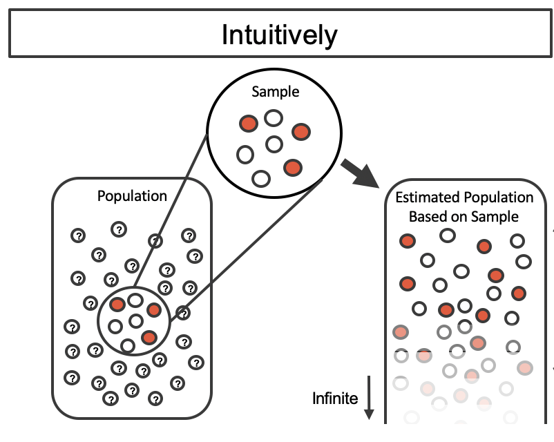
Figure 12.1 shows how the unknown original population can be estimated by using the sample to approximate the proportion of successes and failures (in our case, the proportion of complications and no complications for the medical consultant).
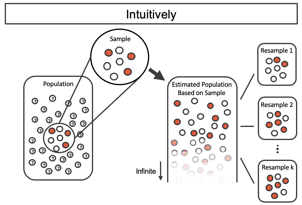
By taking repeated samples from the estimated population, the variability from sample to sample can be observed. In Figure 12.2 the repeated bootstrap samples are obviously different both from each other and from the original population. Recall that the bootstrap samples were taken from the same (estimated) population, and so the differences are due entirely to natural variability in the sampling procedure.
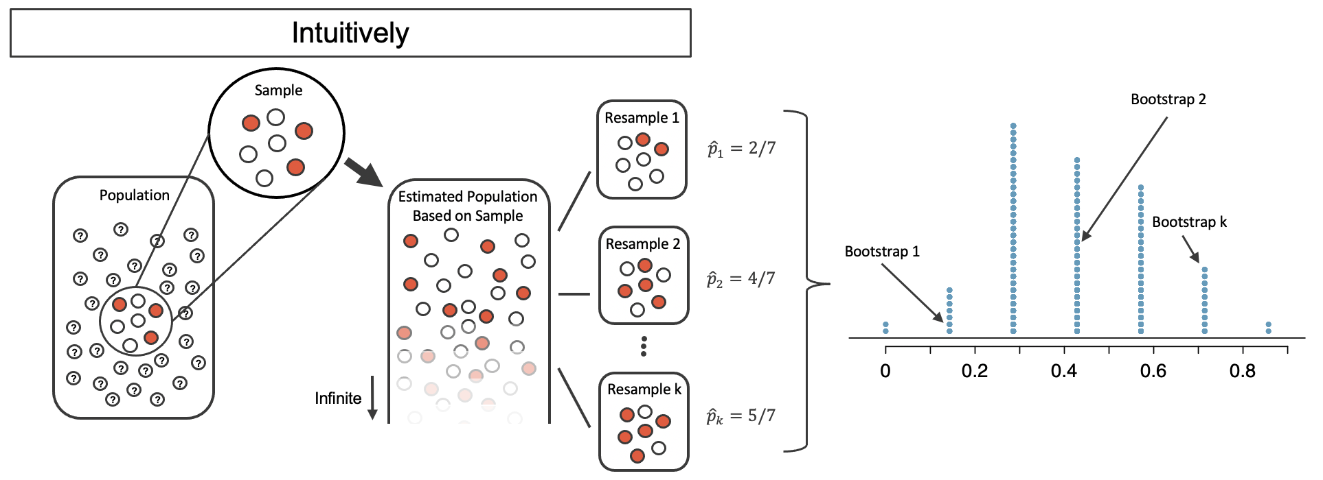
By summarizing each of the bootstrap samples (here, using the sample proportion), we see, directly, the variability of the sample proportion, \(\hat{p},\) from sample to sample. The distribution of \(\hat{p}_{boot}\) for the example scenario is shown in Figure 12.3, and the full bootstrap distribution for the medical consultant data is shown in Figure 12.6.
It turns out that in practice, it is very difficult for computers to work with an infinite population (with the same proportional breakdown as in the sample). However, there is a physical and computational method which produces an equivalent bootstrap distribution of the sample proportion in a computationally efficient manner.
Consider the observed data to be a bag of marbles 3 of which are success (red) and 4 of which are failures (white). By drawing the marbles out of the bag with replacement, we depict the exact same sampling process as was done with the infinitely large estimated population.
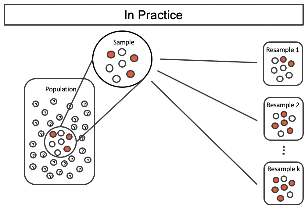
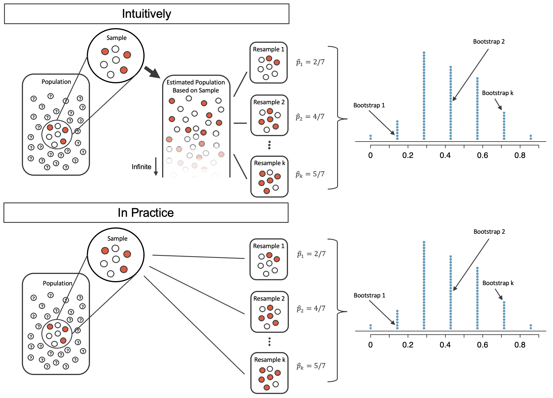
If we apply the bootstrap sampling process to the medical consultant example, we consider each client to be one of the marbles in the bag. There will be 59 white marbles (no complication) and 3 red marbles (complication). If we choose 62 marbles out of the bag (one at a time with replacement) and compute the proportion of simulated patients with complications, \(\hat{p}_{boot},\) then this “bootstrap” proportion represents a single simulated proportion from the “resample from the sample” approach.
In a simulation of 62 patients, about how many would we expect to have had a complication?1
One simulation isn’t enough to get a sense of the variability from one bootstrap proportion to another bootstrap proportion, so we repeat the simulation 10,000 times using a computer.
Figure 12.6 shows the distribution from the 10,000 bootstrap simulations. The bootstrapped proportions vary from about zero to 11.3%. The variability in the bootstrapped proportions leads us to believe that the true probability of complication (the parameter, \(p\)) is likely to fall somewhere between 0% and 11.3%, as these numbers capture 95% of the bootstrap resampled values.
The range of values for the true proportion is called a bootstrap percentile confidence interval, and we will see it again throughout the next few sections and chapters.
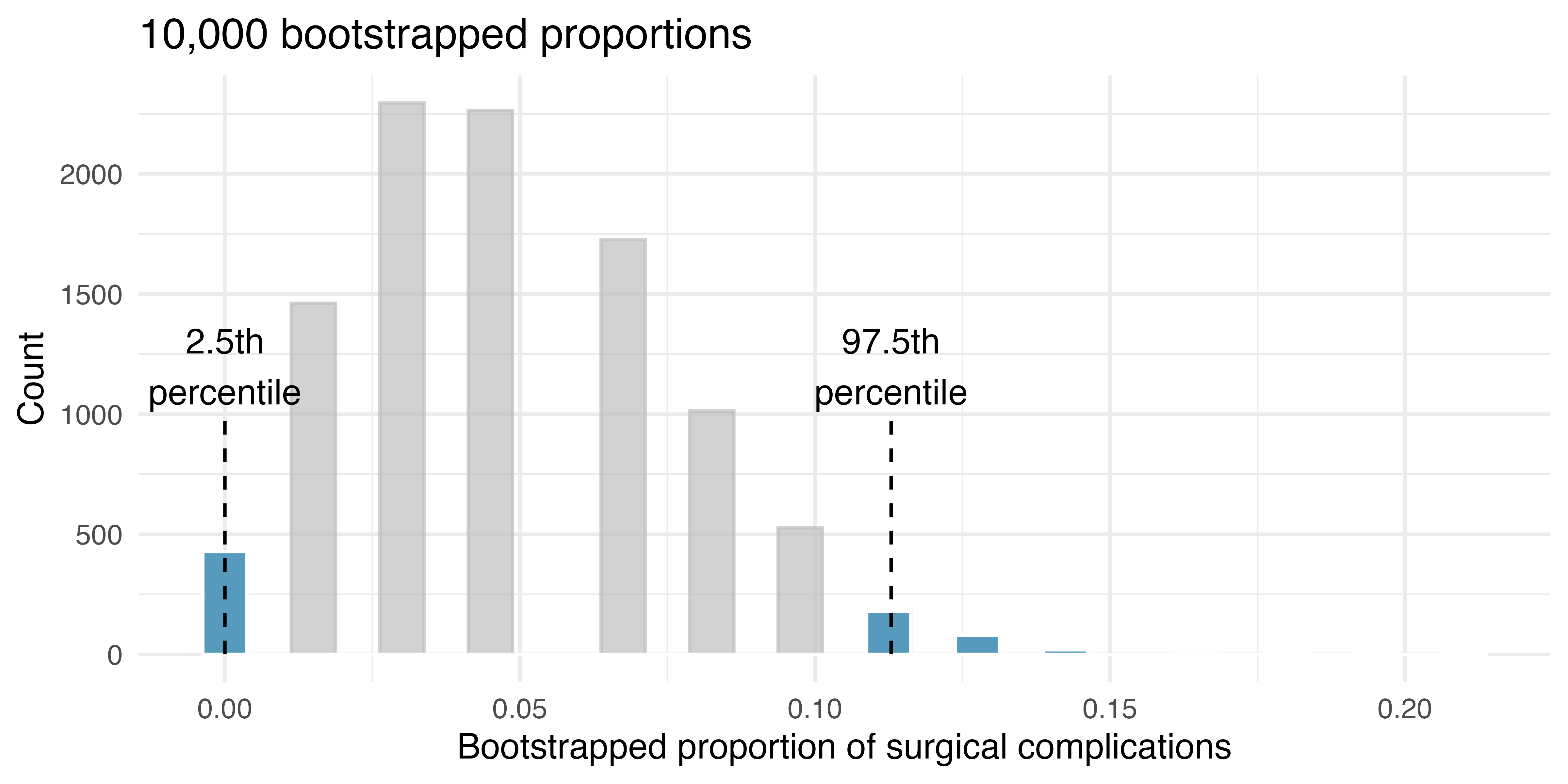
The original claim was that the consultant’s true rate of complication was under the national rate of 10%. Does the interval estimate of 0% to 11.3% for the true probability of complication indicate that the surgical consultant has a lower rate of complications than the national average? Explain.
No. Because the interval overlaps 10%, it might be that the consultant’s work is associated with a lower risk of complications, or it might be that the consultant’s work is associated with a higher risk (i.e., greater than 10%) of complications! Additionally, as previously mentioned, because this is an observational study, even if an association can be measured, there is no evidence that the consultant’s work is the cause of the complication rate (being higher or lower).
12.2 Tappers and listeners case study
Here’s a game you can try with your friends or family: pick a simple, well-known song, tap that tune on your desk, and see if the other person can guess the song. In this simple game, you are the tapper, and the other person is the listener.
12.2.1 Observed data
A Stanford University graduate student named Elizabeth Newton conducted an experiment using the tapper-listener game.2 In her study, she recruited 120 tappers and 120 listeners into the study. About 50% of the tappers expected that the listener would be able to guess the song. Newton wondered, is 50% a reasonable expectation?
In Newton’s study, only 3 out of 120 listeners (\(\hat{p} = 0.025\)) were able to guess the tune! That seems like quite a low number which leads the researcher to ask: what is the true proportion of people who can guess the tune?
12.2.2 Variability of the statistic
To answer the question, we will again use a simulation. To simulate 120 games, this time we use a bag of 120 marbles 3 are red (for those who guessed correctly) and 117 are white (for those who could not guess the song). Sampling from the bag 120 times (remembering to replace the marble back into the bag each time to keep constant the population proportion of red) produces one bootstrap sample.
For example, we can start by simulating 5 tapper-listener pairs by sampling 5 marbles from the bag of 3 red and 117 white marbles.
| W | W | W | R | W |
|---|---|---|---|---|
| Wrong | Wrong | Wrong | Correct | Wrong |
After selecting 120 marbles, we counted 2 red for \(\hat{p}_{boot1} = 0.0167.\) As we did with the randomization technique, seeing what would happen with one simulation isn’t enough. In order to understand how far the observed proportion of 0.025 might be from the true parameter, we should generate more simulations. Here we have repeated the entire simulation ten times:
\[0.0417 \quad 0.025 \quad 0.025 \quad 0.0083 \quad 0.05 \quad 0.0333 \quad 0.025 \quad 0 \quad 0.0083 \quad 0\]
As before, we’ll run a total of 10,000 simulations using a computer. As seen in Figure 12.7, the range of 95% of the resampled values of \(\hat{p}_{boot}\) is 0.000 to 0.0583. That is, we expect that between 0% and 5.83% of people are truly able to guess the tapper’s tune.
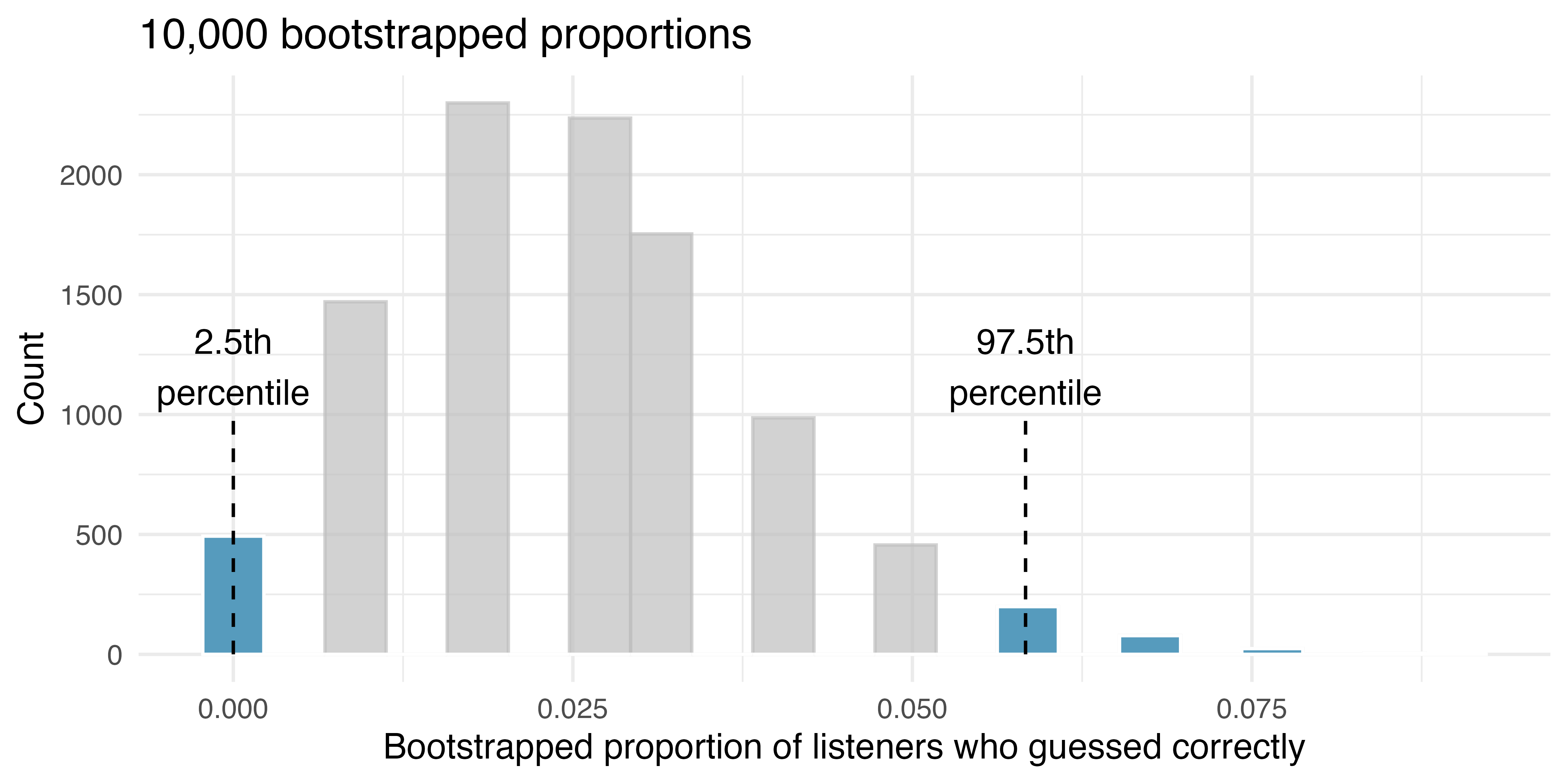
Do the data provide convincing evidence against the claim that 50% of listeners can guess the tapper’s tune?3
12.3 Confidence intervals
A point estimate provides a single plausible value for a parameter. However, a point estimate is rarely perfect; usually there is some error in the estimate. In addition to supplying a point estimate of a parameter, a next logical step would be to provide a plausible range of values for the parameter.
12.3.1 Plausible range of values for the population parameter
A plausible range of values for the population parameter is called a confidence interval. Using only a single point estimate is like fishing in a murky lake with a spear, and using a confidence interval is like fishing with a net. We can throw a spear where we saw a fish, but we will probably miss. On the other hand, if we toss a net in that area, we have a good chance of catching the fish.
If we report a point estimate, we probably will not hit the exact population parameter. On the other hand, if we report a range of plausible values – a confidence interval – we have a good shot at capturing the parameter.
If we want to be very certain we capture the population parameter, should we use a wider interval (e.g., 99%) or a smaller interval (e.g., 80%)?4
12.3.2 Bootstrap confidence interval
As we saw above, a bootstrap sample is a sample of the original sample. In the case of the medical complications data, we proceed as follows:
- Randomly sample one observation from the 62 patients (replace the marble back into the bag so as to keep the population constant).
- Randomly sample a second observation from the 62 patients. Because we sample with replacement (i.e., we do not actually remove the marbles from the bag), there is a 1-in-62 chance that the second observation will be the same one sampled in the first step!
- Keep going one sampled observation at a time …
- Randomly sample the 62nd observation from the 62 patients.
Bootstrap sampling is often called sampling with replacement.
A bootstrap sample behaves similarly to how an actual sample from a population would behave, and we compute the point estimate of interest (here, compute \(\hat{p}_{boot}\)).
Based on theory that is beyond this text, we know that the bootstrap proportions \(\hat{p}_{boot}\) vary around \(\hat{p}\) similarly to how different sample proportions (i.e., values of \(\hat{p}\)) vary around the true parameter \(p.\) Therefore, an interval estimate for \(p\) can be produced using the \(\hat{p}_{boot}\) values themselves.
95% bootstrap percentile confidence interval for a parameter \(p.\)
The 95% bootstrap confidence interval for the parameter \(p\) can be obtained directly using the ordered \(\hat{p}_{boot}\) values.
Consider the sorted \(\hat{p}_{boot}\) values. Call the 2.5% bootstrapped proportion value “lower”, and call the 97.5% bootstrapped proportion value “upper”.
The 95% confidence interval is given by: (lower, upper)
In Section 16.1 we will discuss different percentages for the confidence interval (e.g., 90% confidence interval or 99% confidence interval).
Section Section 16.1 also provides a longer discussion on what “95% confidence” actually means.
12.4 Chapter review
12.4.1 Summary
Figure 12.8 provides a visual summary of creating bootstrap confidence intervals.
We can summarize the bootstrap process as follows:
- Frame the research question in terms of a parameter to estimate. Confidence Intervals are appropriate for research questions that aim to estimate a number from the population (called a parameter).
- Collect data with an observational study or experiment. If a research question can be formed as a query about the parameter, we can collect data to calculate a statistic which is the best guess we have for the value of the parameter. However, we know that the statistic won’t be exactly equal to the parameter due to natural variability.
- Model the randomness by using the data values as a proxy for the population. In order to assess how far the statistic might be from the parameter, we take repeated resamples from the dataset to measure the variability in bootstrapped statistics. The variability of the bootstrapped statistics around the observed statistic (a quantity which can be measured through computational technique) should be approximately the same as the variability of many observed sample statistics around the parameter (a quantity which is very difficult to measure because in real life we only get exactly one sample).
- Create the interval. After choosing a particular confidence level, use the variability of the bootstrapped statistics to create an interval estimate which will hope to capture the true parameter. While the interval estimate associated with the particular sample at hand may or may not capture the parameter, the researcher knows that over their lifetime, the confidence level will determine the percentage of their research confidence intervals that do capture the true parameter.
- Form a conclusion. Using the confidence interval from the analysis, report on the interval estimate for the parameter of interest. Also, be sure to write the conclusion in plain language so casual readers can understand the results.
Table 12.1 is another look at the bootstrap process summary.
| Question | Answer |
|---|---|
| What does it do? | Resamples (with replacement) from the observed data to mimic the sampling variability found by collecting data from a population |
| What is the random process described? | Random sampling from a population |
| What other random processes can be approximated? | Can also be used to describe random allocation in an experiment |
| What is it best for? | Confidence intervals (can also be used for bootstrap hypothesis testing for one proportion as well) |
| What physical object represents the simulation process? | Pulling marbles from a bag with replacement |
12.4.2 Terms
The terms introduced in this chapter are presented in Table 12.2. If you’re not sure what some of these terms mean, we recommend you go back in the text and review their definitions. You should be able to easily spot them as bolded text.
| bootstrap percentile confidence interval | confidence interval | sampling with replacement |
| bootstrap sample | parameter | statistic |
| bootstrapping | point estimate |
12.5 Exercises
Answers to odd-numbered exercises can be found in Appendix A.12.
-
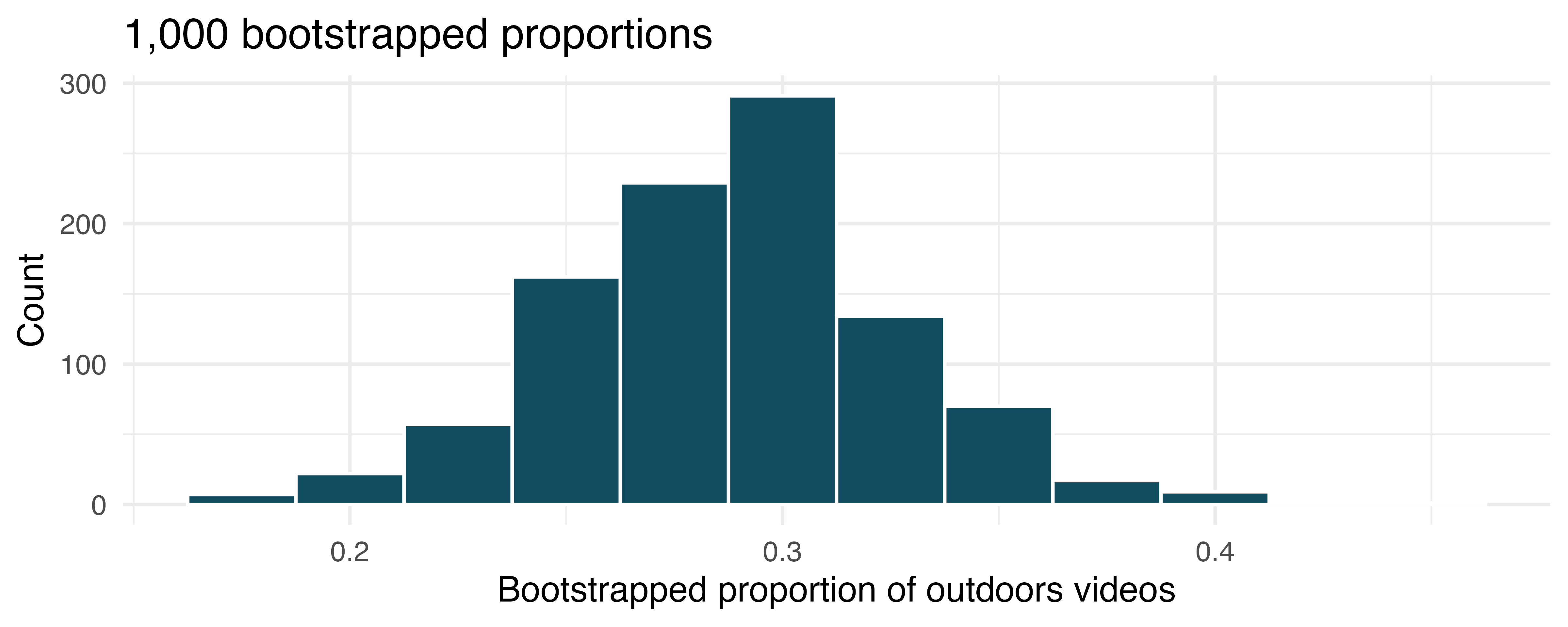
Outside YouTube videos. Let’s say that you want to estimate the proportion of YouTube videos which take place outside (define “outside” to be if any part of the video takes place outdoors). You take a random sample of 128 YouTube videos5 and determine that 37 of them take place outside. You’d like to estimate the proportion of all YouTube videos which take place outside, so you decide to create a bootstrap interval from the original sample of 128 videos.
Describe in words the relevant statistic and parameter for this problem. If you know the numerical value for either one, provide it. If you don’t know the numerical value, explain why the value is unknown.
What notation is used to describe, respectively, the statistic and the parameter?
If using software to bootstrap the original dataset, what is the statistic calculated on each bootstrap sample?
When creating a bootstrap sampling distribution (histogram) of the bootstrapped sample proportions, where should the center of the histogram lie?
The histogram provides a bootstrap sampling distribution for the sample proportion (with 1000 bootstrap repetitions). Using the histogram, estimate a 90% confidence interval for the proportion of YouTube videos which take place outdoors.
Interpret the confidence interval in context of the data.
-
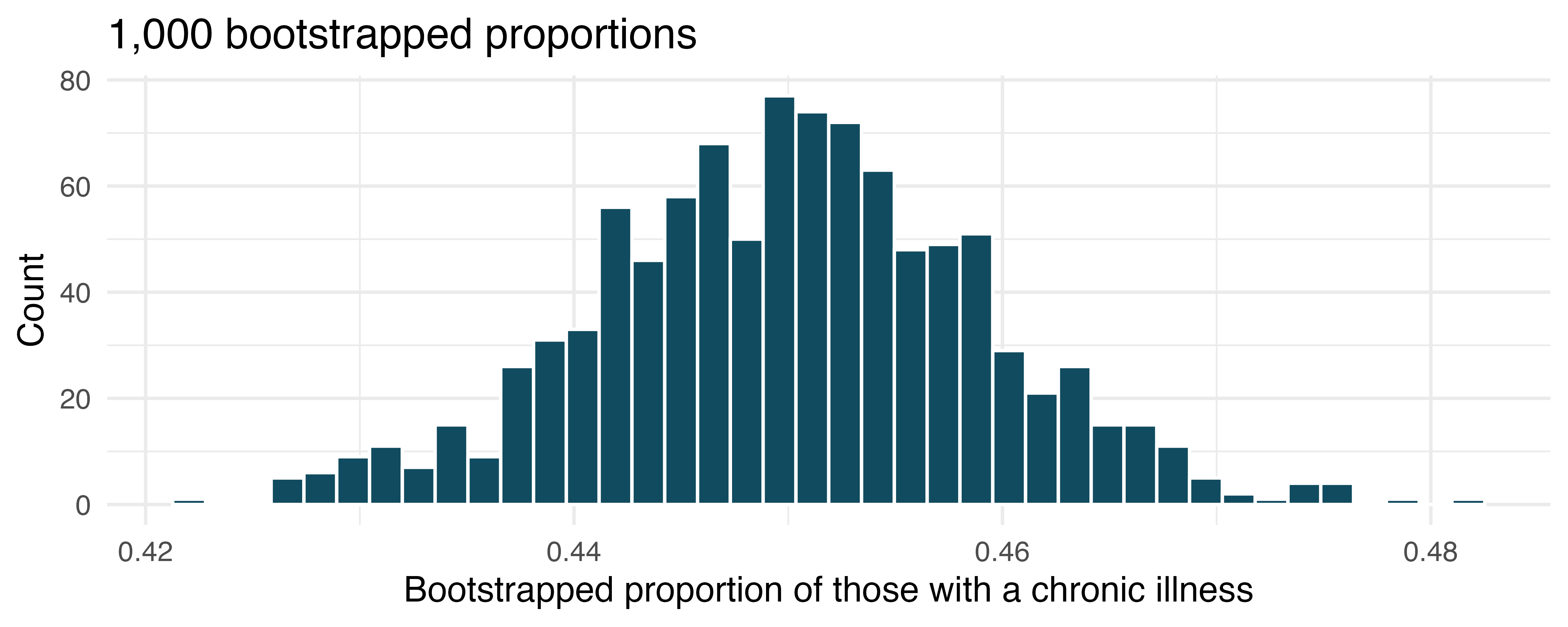
Chronic illness. In 2012 the Pew Research Foundation reported that “45% of US adults report that they live with one or more chronic conditions.” However, this value was based on a sample, so it may not be a perfect estimate for the population parameter of interest on its own. The study was based on a sample of 3014 adults. Below is a distribution of 1000 bootstrapped sample proportions from the Pew dataset. (Pew Research Center 2013) Using the distribution of 1,000 bootstrapped proportions, approximate a 92% confidence interval for the true proportion of US adults who live with one or more chronic conditions and interpret it.
-
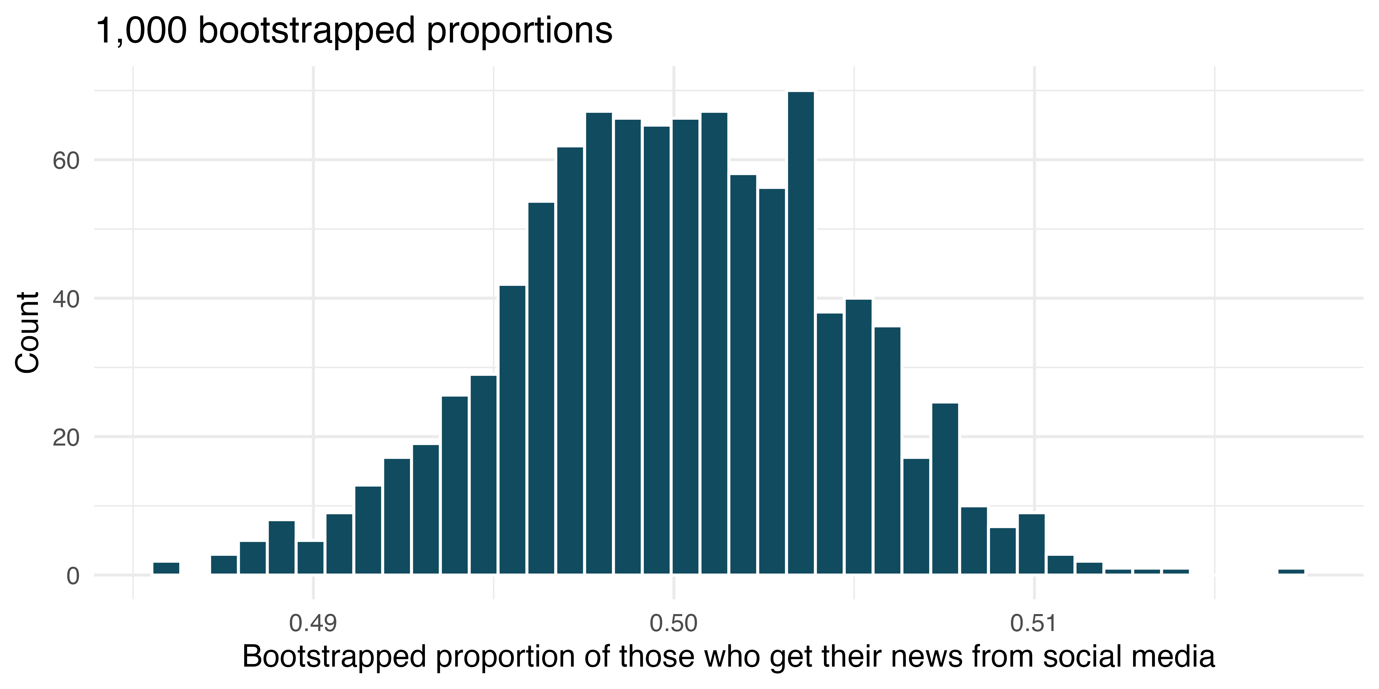
Social media users and news, bootstrapping. A poll conducted in 2022 found that 50% of U.S. adults get news from social media sometimes or often. However, the value was based on a sample, so it may not be a perfect estimate for the population parameter of interest on its own. The study was based on a sample of 12,147 adults. Below is a distribution of 1,000 bootstrapped sample proportions from the Pew dataset. (Pew Research Center 2022) Using the distribution of 1,000 bootstrapped proportions, approximate a 98% confidence interval for the true proportion of US adult social media users (in 2022) who get at least some of their news from Twitter. Interpret the interval in the context of the problem.
-
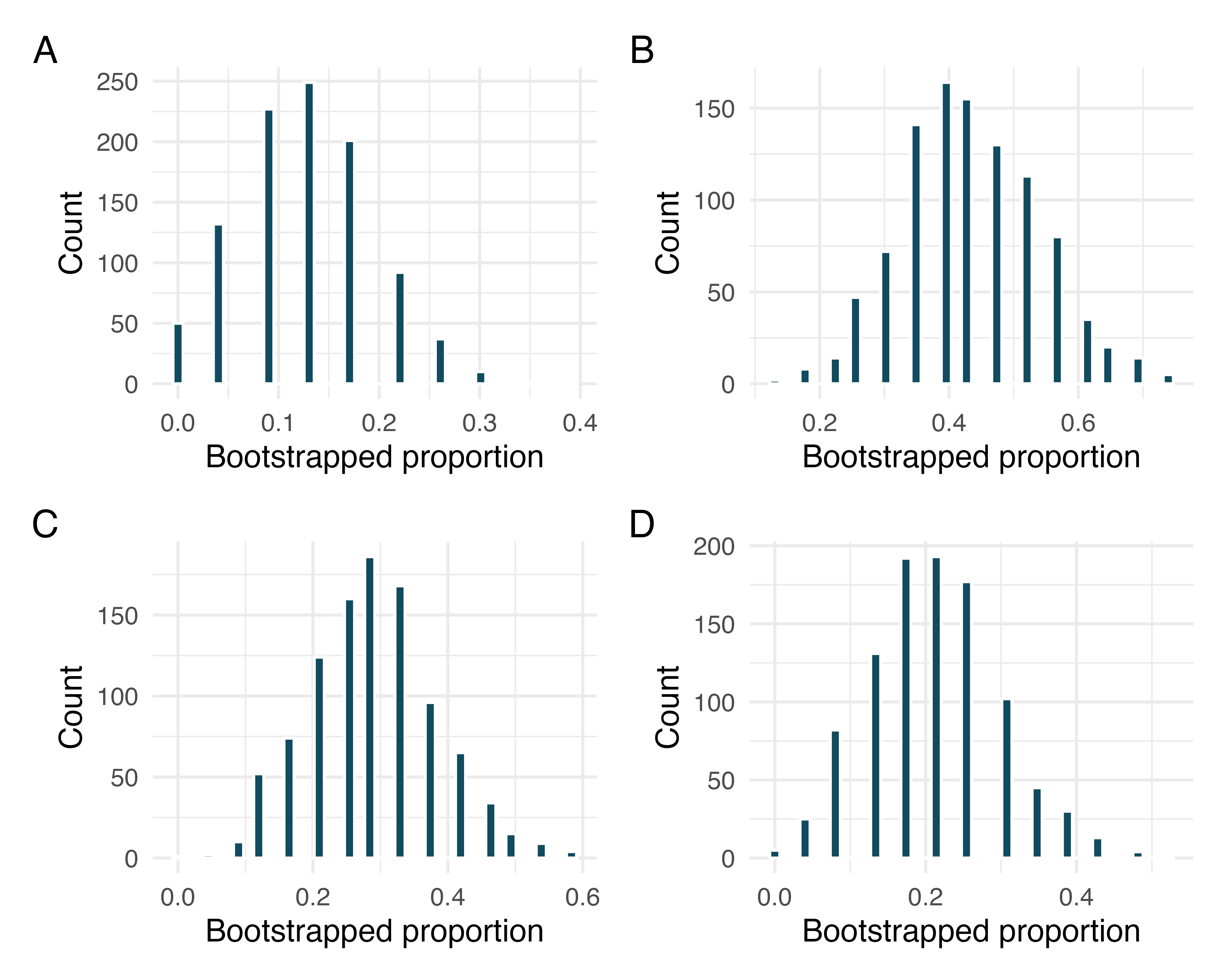
Bootstrap distributions of \(\hat{p}\), I. Each of the following four distributions was created using a different dataset. Each dataset was based on \(n=23\) observations. The original datasets had the following proportions of successes: \[\hat{p} = 0.13 \ \ \hat{p} = 0.22 \ \ \hat{p} = 0.30 \ \ \hat{p} = 0.43.\] Match each histogram with the original data proportion of success.
-
Bootstrap distributions of \(\hat{p}\), II. Each of the following four distributions was created using a different dataset. Each dataset was based on \(n=23\) observations.
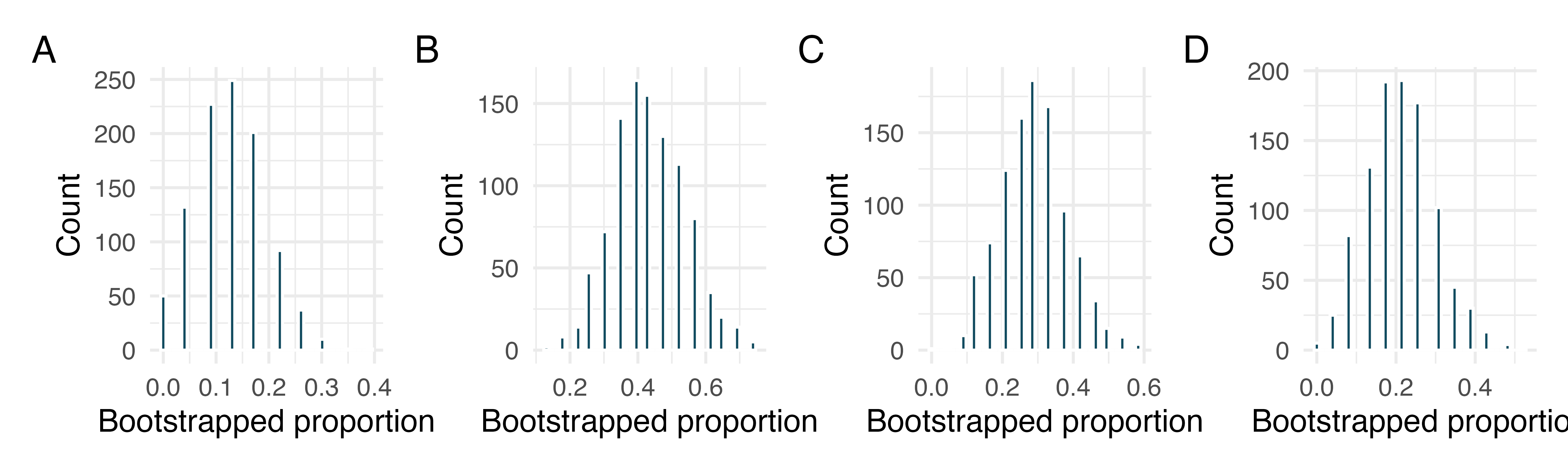
Consider each of the following values for the true popluation \(p\) (proportion of success). Datasets A, B, C, D were bootstrapped 1000 times, with bootstrap proportions as given in the histograms provided. For each parameter value, list the datasets which could plausibly have come from that population. (Hint: there may be more than one dataset for each parameter value.)
\(p = 0.05\)
\(p = 0.25\)
\(p = 0.45\)
\(p = 0.55\)
\(p = 0.75\)
-
Bootstrap distributions of \(\hat{p}\), III. Each of the following four distributions was created using a different dataset. Each dataset had the same proportion of successes \((\hat{p} = 0.4)\) but a different sample size. The four datasets were given by \(n = 10, 100, 500\), and \(1000\).
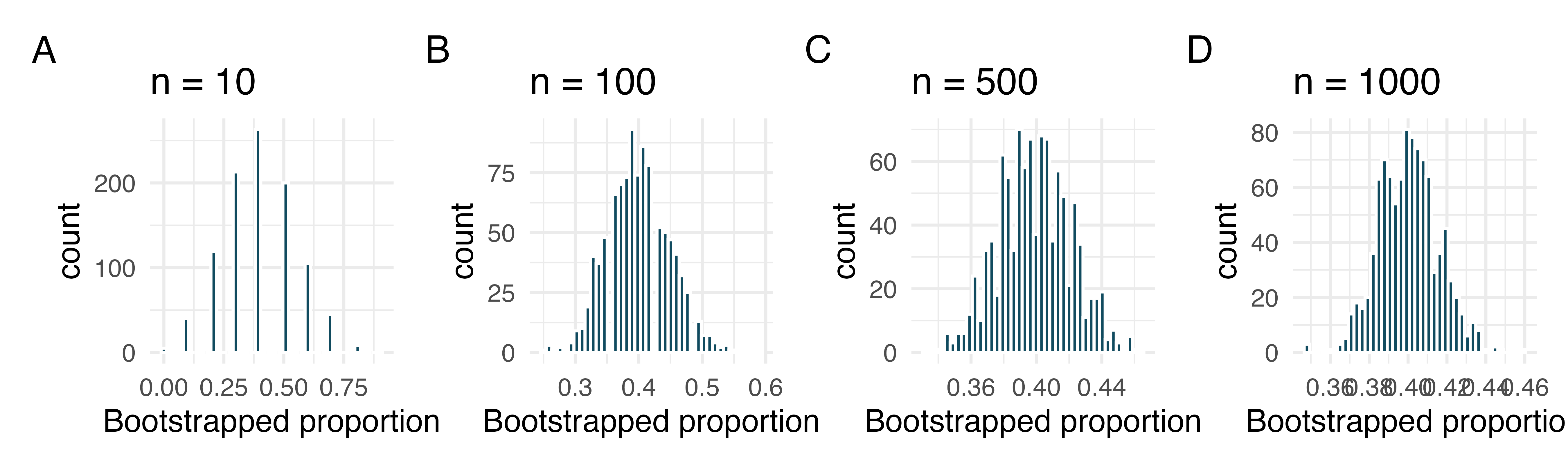
Consider each of the following values for the true popluation \(p\) (proportion of success). Datasets A, B, C, D were bootstrapped 1000 times, with bootstrap proportions as given in the histograms provided. For each parameter value, list the datasets which could plausibly have come from that population. (Hint: there may be more than one dataset for each parameter value.)
\(p = 0.05\)
\(p = 0.25\)
\(p = 0.45\)
\(p = 0.55\)
\(p = 0.75\)
-
Cyberbullying rates. Teens were surveyed about cyberbullying, and 54% to 64% reported experiencing cyberbullying (95% confidence interval). Answer the following questions based on this interval. (Pew Research Center 2018)
A newspaper claims that a majority of teens have experienced cyberbullying. Is this claim supported by the confidence interval? Explain your reasoning.
A researcher conjectured that 70% of teens have experienced cyberbullying. Is this claim supported by the confidence interval? Explain your reasoning.
Without actually calculating the interval, determine if the claim of the researcher from part (b) would be supported based on a 90% confidence interval?
-
Waiting at an ER. A 95% confidence interval for the mean waiting time at an emergency room (ER) of (128 minutes, 147 minutes). Answer the following questions based on this interval.
A local newspaper claims that the average waiting time at this ER exceeds 3 hours. Is this claim supported by the confidence interval? Explain your reasoning.
The Dean of Medicine at this hospital claims the average wait time is 2.2 hours. Is this claim supported by the confidence interval? Explain your reasoning.
Without actually calculating the interval, determine if the claim of the Dean from part (b) would be supported based on a 99% confidence interval?
About 4.8% of the patients (3 on average) in the simulation will have a complication, as this is what was seen in the sample. We will, however, see a little variation from one simulation to the next.↩︎
This case study is described in Made to Stick by Chip and Dan Heath. Little known fact: the teaching principles behind many OpenIntro resources are based on Made to Stick.↩︎
Because 50% is not in the interval estimate for the true parameter, we can say that there is convincing evidence against the hypothesis that 50% of listeners can guess the tune. Moreover, 50% is a substantial distance from the largest resample statistic, suggesting that there is very convincing evidence against this hypothesis.↩︎
If we want to be more certain we will capture the fish, we might use a wider net. Likewise, we use a wider confidence interval if we want to be more certain that we capture the parameter.↩︎
There are many choices for implementing a random selection of YouTube videos, but it isn’t clear how “random” they are.↩︎