14 Decision Errors
Using data to make inferential decisions about larger populations is not a perfect process. As seen in Chapter 11, a small p-value typically leads the researcher to a decision to reject the null claim or hypothesis. Sometimes, however, data can produce a small p-value when the null hypothesis is actually true and the data are just inherently variable. Here we describe the errors which can arise in hypothesis testing, how to define and quantify the different errors, and suggestions for mitigating errors if possible.
Hypothesis tests are not flawless. Just think of the court system: innocent people are sometimes wrongly convicted and the guilty sometimes walk free. Similarly, data can point to the wrong conclusion. However, what distinguishes statistical hypothesis tests from a court system is that our framework allows us to quantify and control how often the data lead us to the incorrect conclusion.
In a hypothesis test, there are two competing hypotheses: the null and the alternative. We make a statement about which one might be true, but we might choose incorrectly. There are four possible scenarios in a hypothesis test, which are summarized in Table 14.1.
| Truth | Reject null hypothesis | Fail to reject null hypothesis |
|---|---|---|
| Null hypothesis is true | Type I error | Good decision |
| Alternative hypothesis is true | Good decision | Type II error |
A Type I error is rejecting the null hypothesis when \(H_0\) is actually true. Since we rejected the null hypothesis in the sex discrimination and opportunity cost studies, it is possible that we made a Type I error in one or both of those studies. A Type II error is failing to reject the null hypothesis when the alternative is actually true.
In a US court, the defendant is either innocent \((H_0)\) or guilty \((H_A).\) What does a Type I error represent in this context? What does a Type II error represent? Table 14.1 may be useful.
If the court makes a Type I error, this means the defendant is innocent \((H_0\) true) but wrongly convicted. A Type II error means the court failed to reject \(H_0\) (i.e., failed to convict the person) when they were in fact guilty \((H_A\) true).
Consider the opportunity cost study where we concluded students were less likely to make a DVD purchase if they were reminded that money not spent now could be spent later. What would a Type I error represent in this context?1
How could we reduce the Type I error rate in US courts? What influence would this have on the Type II error rate?
To lower the Type I error rate, we might raise our standard for conviction from “beyond a reasonable doubt” to “beyond a conceivable doubt” so fewer people would be wrongly convicted. However, this would also make it more difficult to convict the people who are actually guilty, so we would make more Type II errors.
How could we reduce the Type II error rate in US courts? What influence would this have on the Type I error rate?2
The example and guided practice above provide an important lesson: if we reduce how often we make one type of error, we generally make more of the other type.
14.1 Discernibility level
The discernibility level provides the cutoff for the p-value which will lead to a decision of “reject the null hypothesis.” Choosing a discernibility level for a test is important in many contexts, and the traditional level is 0.05. However, it is sometimes helpful to adjust the discernibility level based on the application. We may select a level that is smaller or larger than 0.05 depending on the consequences of any conclusions reached from the test.
If making a Type I error is dangerous or especially costly, we should choose a small discernibility level (e.g., 0.01 or 0.001). If we want to be very cautious about rejecting the null hypothesis, we demand very strong evidence favoring the alternative \(H_A\) before we would reject \(H_0.\)
If a Type II error is relatively more dangerous or much more costly than a Type I error, then we should choose a higher discernibility level (e.g., 0.10). Here we want to be cautious about failing to reject \(H_0\) when the null is actually false.
Discernibility levels should reflect consequences of errors.
The discernibility level selected for a test should reflect the real-world consequences associated with making a Type I or Type II error.
14.2 Two-sided hypotheses
In Chapter 11 we explored whether women were discriminated against and whether a simple trick could make students a little thriftier. In these two case studies, we have actually ignored some possibilities:
- What if men are actually discriminated against?
- What if the money trick actually makes students spend more?
These possibilities weren’t considered in our original hypotheses or analyses. The disregard of the extra alternatives may have seemed natural since the data pointed in the directions in which we framed the problems. However, there are two dangers if we ignore possibilities that disagree with our data or that conflict with our world view:
Framing an alternative hypothesis simply to match the direction that the data point will generally inflate the Type I error rate. After all the work we have done (and will continue to do) to rigorously control the error rates in hypothesis tests, careless construction of the alternative hypotheses can disrupt that hard work.
If we only use alternative hypotheses that agree with our worldview, then we are going to be subjecting ourselves to confirmation bias, which means we are looking for data that supports our ideas. That’s not very scientific, and we can do better!
The original hypotheses we have seen are called one-sided hypothesis tests because they only explored one direction of possibilities. Such hypotheses are appropriate when we are exclusively interested in the single direction, but usually we want to consider all possibilities. To do so, let’s learn about two-sided hypothesis tests in the context of a new study that examines the impact of using blood thinners on patients who have undergone CPR.
Cardiopulmonary resuscitation (CPR) is a procedure used on individuals suffering a heart attack when other emergency resources are unavailable. This procedure is helpful in providing some blood circulation to keep a person alive, but CPR chest compression can also cause internal injuries. Internal bleeding and other injuries that can result from CPR complicate additional treatment efforts. For instance, blood thinners may be used to help release a clot that is causing the heart attack once a patient arrives in the hospital. However, blood thinners negatively affect internal injuries.
Here we consider an experiment with patients who underwent CPR for a heart attack and were subsequently admitted to a hospital. Each patient was randomly assigned to either receive a blood thinner (treatment group) or not receive a blood thinner (control group). The outcome variable of interest was whether the patient survived for at least 24 hours. (Böttiger et al. 2001)
Form hypotheses for this study in plain and statistical language. Let \(p_C\) represent the true survival rate of people who do not receive a blood thinner (corresponding to the control group) and \(p_T\) represent the survival rate for people receiving a blood thinner (corresponding to the treatment group).
We want to understand whether blood thinners are helpful or harmful. We’ll consider both of these possibilities using a two-sided hypothesis test.
\(H_0:\) Blood thinners do not have an overall survival effect, i.e., the survival proportions are the same in each group. \(p_T - p_C = 0.\)
\(H_A:\) Blood thinners have an impact on survival, either positive or negative, but not zero. \(p_T - p_C \neq 0.\)
Note that if we had done a one-sided hypothesis test, the resulting hypotheses would have been:
\(H_0:\) Blood thinners do not have a positive overall survival effect, i.e., the survival proportions for the blood thinner group is the same or lower than the control group. \(p_T - p_C \leq 0.\)
\(H_A:\) Blood thinners have a positive impact on survival. \(p_T - p_C > 0.\)
There were 50 patients in the experiment who did not receive a blood thinner and 40 patients who did. The study results are shown in Table 14.2.
| Group | Died | Survived | Total |
|---|---|---|---|
| Control | 39 | 11 | 50 |
| Treatment | 26 | 14 | 40 |
| Total | 65 | 25 | 90 |
What is the observed survival rate in the control group? And in the treatment group? Also, provide a point estimate \((\hat{p}_T - \hat{p}_C)\) for the true difference in population survival proportions across the two groups: \(p_T - p_C.\)3
According to the point estimate, for patients who have undergone CPR outside of the hospital, an additional 13% of these patients survive when they are treated with blood thinners. However, we wonder if this difference could be easily explainable by chance, if the treatment has no effect on survival.
As we did in past studies, we will simulate what type of differences we might see from chance alone under the null hypothesis. By randomly assigning each of the patient’s files to a “simulated treatment” or “simulated control” allocation, we get a new grouping. If we repeat this simulation 1,000 times, we can build a null distribution of the differences shown in Figure 14.1.
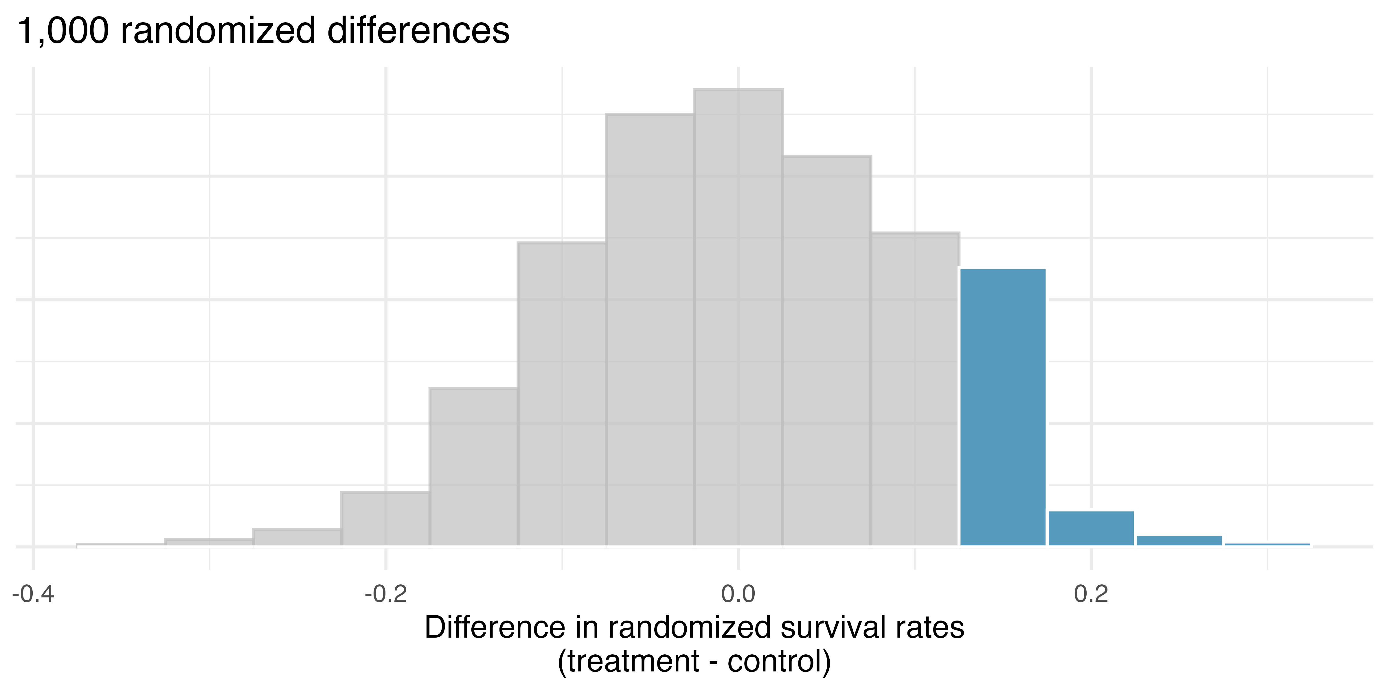
The right tail area is 0.135. (Note: it is only a coincidence that we also have \(\hat{p}_T - \hat{p}_C=0.13.)\) However, contrary to how we calculated the p-value in previous studies, the p-value of this test is not actually the tail area we calculated, i.e., it’s not 0.135!
The p-value is defined as the probability we observe a result at least as favorable to the alternative hypothesis as the observed difference. In this case, any differences less than or equal to -0.13 would also provide equally strong evidence favoring the alternative hypothesis as a difference of +0.13 did. A difference of -0.13 would correspond to 13% higher survival rate in the control group than the treatment group. In Figure 14.2 we have also shaded these differences in the left tail of the distribution. These two shaded tails provide a visual representation of the p-value for a two-sided test.
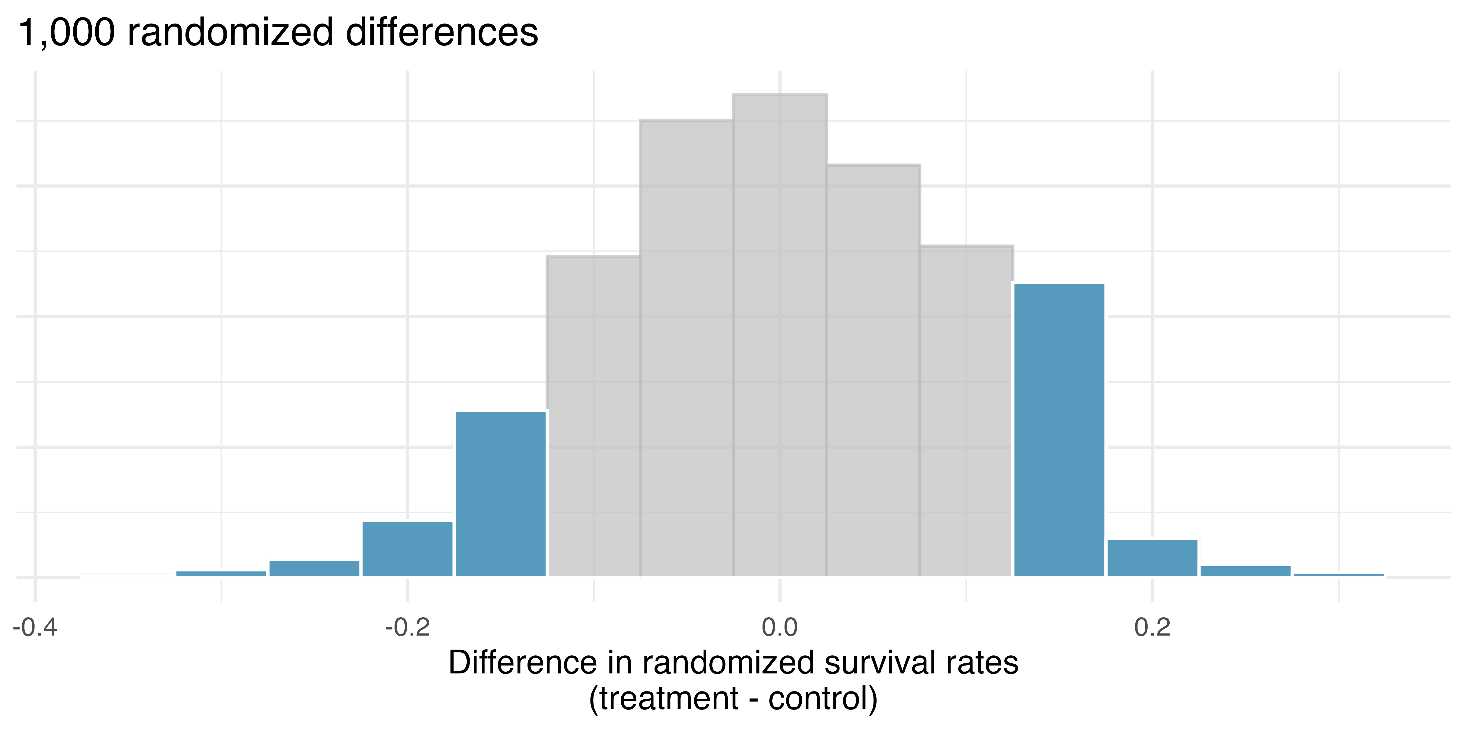
For a two-sided test, take the single tail (in this case, 0.131) and double it to get the p-value: 0.262. Since this p-value is larger than 0.05, we do not reject the null hypothesis. That is, we do not find convincing evidence that the blood thinner has any influence on survival of patients who undergo CPR prior to arriving at the hospital.
Default to a two-sided test.
We want to be rigorous and keep an open mind when we analyze data and evidence. Use a one-sided hypothesis test only if you truly have interest in only one direction.
Computing a p-value for a two-sided test.
First compute the p-value for one tail of the distribution, then double that value to get the two-sided p-value. That’s it!
Consider the situation of the medical consultant. Now that you know about one-sided and two-sided tests, which type of test do you think is more appropriate?
The setting has been framed in the context of the consultant being helpful (which is what led us to a one-sided test originally), but what if the consultant actually performed worse than the average? Would we care? More than ever! Since it turns out that we care about a finding in either direction, we should run a two-sided test. The p-value for the two-sided test is double that of the one-sided test, here the simulated p-value would be 0.2444.
Generally, to find a two-sided p-value we double the single tail area, which remains a reasonable approach even when the distribution is asymmetric. However, the approach can result in p-values larger than 1 when the point estimate is very near the mean in the null distribution; in such cases, we write that the p-value is 1. Also, very large p-values computed in this way (e.g., 0.85), may also be slightly inflated. Typically, we do not worry too much about the precision of very large p-values because they lead to the same analysis conclusion, even if the value is slightly off.
14.3 Controlling the Type I error rate
Now that we understand the difference between one-sided and two-sided tests, we must recognize when to use each type of test. Because of the result of increased error rates, it is never okay to change two-sided tests to one-sided tests after observing the data. We explore the consequences of ignoring this advice in the next example.
Using \(\alpha=0.05,\) we show that freely switching from two-sided tests to one-sided tests will lead us to make twice as many Type I errors as intended.
Suppose we are interested in finding any difference from 0. We’ve created a smooth-looking null distribution representing differences due to chance below.
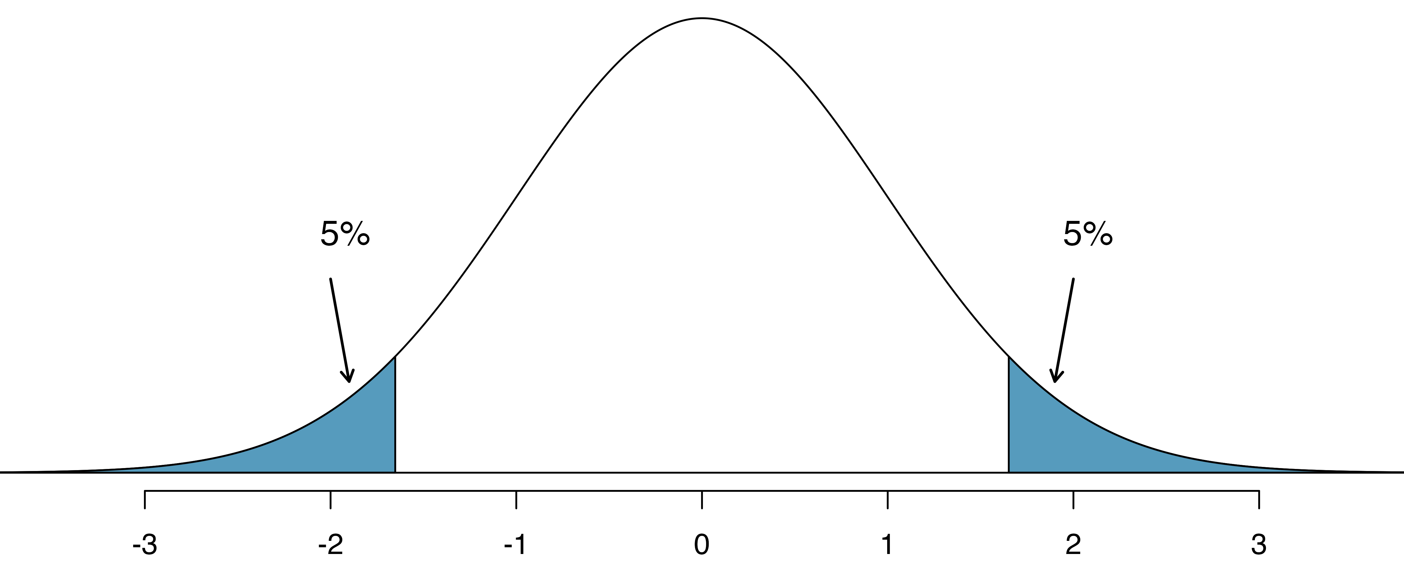
First, suppose the sample difference was larger than 0. In a one-sided test, we would set \(H_A:\) difference \(> 0.\) If the observed difference falls in the upper 5% of the distribution, we would reject \(H_0\) since the p-value would just be the single tail. Thus, if \(H_0\) is true, we incorrectly reject \(H_0\) about 5% of the time when the sample mean is above the null value, as shown above.
Then, suppose the sample difference was smaller than 0. In a one-sided test, we would set \(H_A:\) difference \(< 0.\) If the observed difference falls in the lower 5% of the figure, we would reject \(H_0.\) That is, if \(H_0\) is true, then we would observe this situation about 5% of the time.
By examining these two scenarios, we can determine that we will make a Type I error \(5\%+5\%=10\%\) of the time if we are allowed to swap to the “best” one-sided test for the data. This is twice the error rate we prescribed with our discernibility level: \(\alpha=0.05\)!
Hypothesis tests should be set up before seeing the data.
After observing data, it is tempting to turn a two-sided test into a one-sided test. Avoid this temptation. Hypotheses should be set up before observing the data.
14.4 Power
Although we won’t go into extensive detail here, power is an important topic for follow-up consideration after understanding the basics of hypothesis testing. A good power analysis is a vital preliminary step to any study as it will inform whether the data you collect are sufficient for being able to conclude your research broadly.
Often times in experiment planning, there are two competing considerations:
- We want to collect enough data that we can detect important effects.
- Collecting data can be expensive, and, in experiments involving people, there may be some risk to patients.
When planning a study, we want to know how likely we are to detect an effect we care about. In other words, if there is a real effect, and that effect is large enough that it has practical value, then what is the probability that we detect that effect? This probability is called the power, and we can compute it for different sample sizes or different effect sizes.
Power.
The power of the test is the probability of rejecting the null claim when the alternative claim is true.
How easy it is to detect the effect depends on both how big the effect is (e.g., how good the medical treatment is) as well as the sample size.
We think of power as the probability that you will become rich and famous from your science. In order for your science to make a splash, you need to have good ideas! That is, you won’t become famous if you happen to find a single Type I error which rejects the null hypothesis. Instead, you’ll become famous if your science is very good and important (that is, if the alternative hypothesis is true). The better your science is (i.e., the better the medical treatment), the larger the effect size and the easier it will be for you to convince people of your work.
Not only does your science need to be solid, but you also need to have evidence (i.e., data) that shows the effect. A few observations (e.g., \(n = 2)\) is unlikely to be convincing because of well known ideas of natural variability. Indeed, the larger the dataset which provides evidence for your scientific claim, the more likely you are to convince the community that your idea is correct.
Although a full discussion of relative power is beyond the scope of this text, you might be interested to know that, often, paired t-tests (discussed in Section 21.3) are more powerful than independent t-tests (discussed in Section 20.3) because the pairing reduces the inherent variability across observations. Additionally, because the median is almost always more variable than the mean, tests based on the mean are more powerful than tests based on the median. That is to say, reducing variability (done in different ways depending on the experimental design and set-up of the analysis) makes a test more powerful in such that the data are more likely to reject the null hypothesis.
14.5 Chapter review
14.5.1 Summary
Although hypothesis testing provides a strong framework for making decisions based on data, as the analyst, you need to understand how and when the process can go wrong. That is, always keep in mind that the conclusion to a hypothesis test may not be right! Sometimes when the null hypothesis is true, we will accidentally reject it and commit a Type I error; sometimes when the alternative hypothesis is true, we will fail to reject the null hypothesis and commit a Type II error. The power of the test quantifies how likely it is to obtain data which will reject the null hypothesis when indeed the alternative is true; the power of the test is increased when larger sample sizes are taken.
14.5.2 Terms
The terms introduced in this chapter are presented in Table 14.3. If you’re not sure what some of these terms mean, we recommend you go back in the text and review their definitions. You should be able to easily spot them as bolded text.
| confirmation bias | one-sided hypothesis test | two-sided hypothesis test |
| discernibility level | power | Type I error |
| null distribution | significance level | Type II error |
14.6 Exercises
Answers to odd-numbered exercises can be found in Appendix A.14.
-
Testing for Fibromyalgia. A patient named Diana was diagnosed with Fibromyalgia, a long-term syndrome of body pain, and was prescribed anti-depressants. Being the skeptic that she is, Diana didn’t initially believe that anti-depressants would help her symptoms. However after a couple months of being on the medication she decides that the anti-depressants are working, because she feels like her symptoms are in fact getting better.
Write the hypotheses in words for Diana’s skeptical position when she started taking the anti-depressants.
What is a Type I error in this context?
What is a Type II error in this context?
-
Testing for food safety. A food safety inspector is called upon to investigate a restaurant with a few customer reports of poor sanitation practices. The food safety inspector uses a hypothesis testing framework to evaluate whether regulations are not being met. If he decides the restaurant is in gross violation, its license to serve food will be revoked.
Write the hypotheses in words.
What is a Type I error in this context?
What is a Type II error in this context?
Which error is more problematic for the restaurant owner? Why?
Which error is more problematic for the diners? Why?
As a diner, would you prefer that the food safety inspector requires strong evidence or very strong evidence of health concerns before revoking a restaurant’s license? Explain your reasoning.
-
Which is higher? In each part below, there is a value of interest and two scenarios: (i) and (ii). For each part, report if the value of interest is larger under scenario (i), scenario (ii), or whether the value is equal under the scenarios.
The standard error of \(\hat{p}\) when (i) \(n = 125\) or (ii) \(n = 500\).
The margin of error of a confidence interval when the confidence level is (i) 90% or (ii) 80%.
The p-value for a Z-statistic of 2.5 calculated based on a (i) sample with \(n = 500\) or based on a (ii) sample with \(n = 1000\).
The probability of making a Type II error when the alternative hypothesis is true and the discernibility level is (i) 0.05 or (ii) 0.10.
-
True / False. Determine if the following statements are true or false, and explain your reasoning. If false, state how it could be corrected.
If a given value (for example, the null hypothesized value of a parameter) is within a 95% confidence interval, it will also be within a 99% confidence interval.
Decreasing the discernibility level (\(\alpha\)) will increase the probability of making a Type I error.
Suppose the null hypothesis is \(p = 0.5\) and we fail to reject \(H_0\). Under this scenario, the true population proportion is 0.5.
With large sample sizes, even small differences between the null value and the observed point estimate, a difference often called the effect size, will be identified as statistically discernible.
-
Online communication. A study suggests that 60% of college student spend 10 or more hours per week communicating with others online. You believe that this is incorrect and decide to collect your own sample for a hypothesis test. You randomly sample 160 students from your dorm and find that 70% spent 10 or more hours a week communicating with others online. A friend of yours, who offers to help you with the hypothesis test, comes up with the following set of hypotheses. Indicate any errors you see.
\[H_0: \hat{p} < 0.6 \quad \quad H_A: \hat{p} > 0.7\]
- Same observation, different sample size. Suppose you conduct a hypothesis test based on a sample where the sample size is \(n = 50\), and arrive at a p-value of 0.08. You then refer back to your notes and discover that you made a careless mistake, the sample size should have been \(n = 500\). Will your p-value increase, decrease, or stay the same? Explain.
- Estimating \(\pi\). In a class activity, each of 100 students experimentally estimates the value of \(\pi\), 10 separate times. Using the 10 measurements for \(\pi\) (10 values of \(\hat{\pi}\)), each student calculates a confidence interval for \(\pi\). In grading the 100 student assignments, the professor marks 7 of the assignments wrong, indicating that the 7 students must have done their experiments or analysis incorrectly because each of the 7 students reported confidence intervals that did not capture the known true value of \(\pi\), roughly 3.14159. Was the professor correct to mark the assignments wrong for having CIs that did not capture the value of 3.14159? Explain.4
-
Fermenting yeast. Twenty students work individually in a biology lab to test whether using raw sucrose versus refined sugar will lead to the same yeast fermentation rate. Each student runs a full experiment independently of the other students in the lab. Of the twenty students, twelve are able to reject the null hypothesis and to claim that the fermentation rates are different.5
- Explain what type of error was likely to have occurred in this situation.
- What change would you suggest that would lower the error rate?
- Practical importance vs. statistical discernibility. Determine whether the following statement is true or false, and explain your reasoning: “With large sample sizes, even small differences between the null value and the observed point estimate can be statistically discernible.”
-
Hypothesis statements. For each of the research claims below, fill in the value and the direction of the null and alternative hypotheses. That is, complete all aspects of the following hypothesis statements. Additionally, for each item, describe \(p\) in words.
\[H_0: p \_\_\_\_ \_\_\_\_ \quad \quad H_A: p \_\_\_\_ \_\_\_\_\]
On a pre-test to assess knowledge of the upcoming material, a professor wants to determine if their students know, on average, more than if they were just randomly guessing. The pre-test is 30 multiple choice questions, where each question has 5 possible responses.
A standard treatment is known to reduce blood pressure in 32% of patients. A clinical trial is conducted to assess whether a new medical intervention will produce results which are different than the standard treatment, in terms of the percent of patients who will have reduced blood pressure.
In the last presidential election 67% of registered voters turned out to vote. Will the next presidential election have a higher turn-out of voters?
Making a Type I error in this context would mean that reminding students that money not spent now can be spent later does not affect their buying habits, despite the strong evidence (the data suggesting otherwise) found in the experiment. Notice that this does not necessarily mean something was wrong with the data or that we made a computational mistake. Sometimes data simply point us to the wrong conclusion, which is why scientific studies are often repeated to check initial findings.↩︎
To lower the Type II error rate, we want to convict more guilty people. We could lower the standards for conviction from “beyond a reasonable doubt” to “beyond a little doubt”. Lowering the bar for guilt will also result in more wrongful convictions, raising the Type I error rate.↩︎
Observed control survival rate: \(\hat{p}_C = \frac{11}{50} = 0.22.\) Treatment survival rate: \(\hat{p}_T = \frac{14}{40} = 0.35.\) Observed difference: \(\hat{p}_T - \hat{p}_C = 0.35 - 0.22 = 0.13.\)↩︎
This exercise was inspired by discussion with Dr. Annelise Wagner.↩︎
This exercise was inspired by discussion with Dr. Annelise Wagner.↩︎