20 Inference for comparing two independent means
We now extend the methods from Chapter 19 to apply confidence intervals and hypothesis tests to differences in population means that come from two groups, Group 1 and Group 2: \(\mu_1 - \mu_2.\)
In our investigations, we’ll identify a reasonable point estimate of \(\mu_1 - \mu_2\) based on the sample, and you may have already guessed its form: \(\bar{x}_1 - \bar{x}_2.\) Then we’ll look at the inferential analysis in three different ways: using a randomization test, applying bootstrapping for interval estimates, and, if we verify that the point estimate can be modeled using a normal distribution, we compute the estimate’s standard error and apply the mathematical framework.
In this section we consider a difference in two population means, \(\mu_1 - \mu_2,\) under the condition that the data are not paired. Just as with a single sample, we identify conditions to ensure we can use the \(t\)-distribution with a point estimate of the difference, \(\bar{x}_1 - \bar{x}_2,\) and a new standard error formula.
The details for working through inferential problems in the two independent means setting are strikingly similar to those applied to the two independent proportions setting. We first cover a randomization test where the observations are shuffled under the assumption that the null hypothesis is true. Then we bootstrap the data (with no imposed null hypothesis) to create a confidence interval for the true difference in population means, \(\mu_1 - \mu_2.\) The mathematical model, here the \(t\)-distribution, is able to describe both the randomization test and the bootstrapping as long as the conditions are met.
The inferential tools are applied to three different data contexts: determining whether stem cells can improve heart function, exploring the relationship between pregnant women’s smoking habits and birth weights of newborns, and exploring whether there is convincing evidence that one variation of an exam is harder than another variation. This section is motivated by questions like “Is there convincing evidence that newborns from mothers who smoke have a different average birth weight than newborns from mothers who do not smoke?”
20.1 Randomization test for the difference in means
An instructor decided to run two slight variations of the same exam. Prior to passing out the exams, they shuffled the exams together to ensure each student received a random version. Anticipating complaints from students who took Version B, they would like to evaluate whether the difference observed in the groups is so large that it provides convincing evidence that Version B was more difficult (on average) than Version A.
20.1.1 Observed data
Summary statistics for how students performed on these two exams are shown in Table 20.1 and plotted in Figure 20.1.
| Group | n | Mean | SD | Min | Max |
|---|---|---|---|---|---|
| A | 58 | 75.1 | 13.9 | 44 | 100 |
| B | 55 | 72.0 | 13.8 | 38 | 100 |
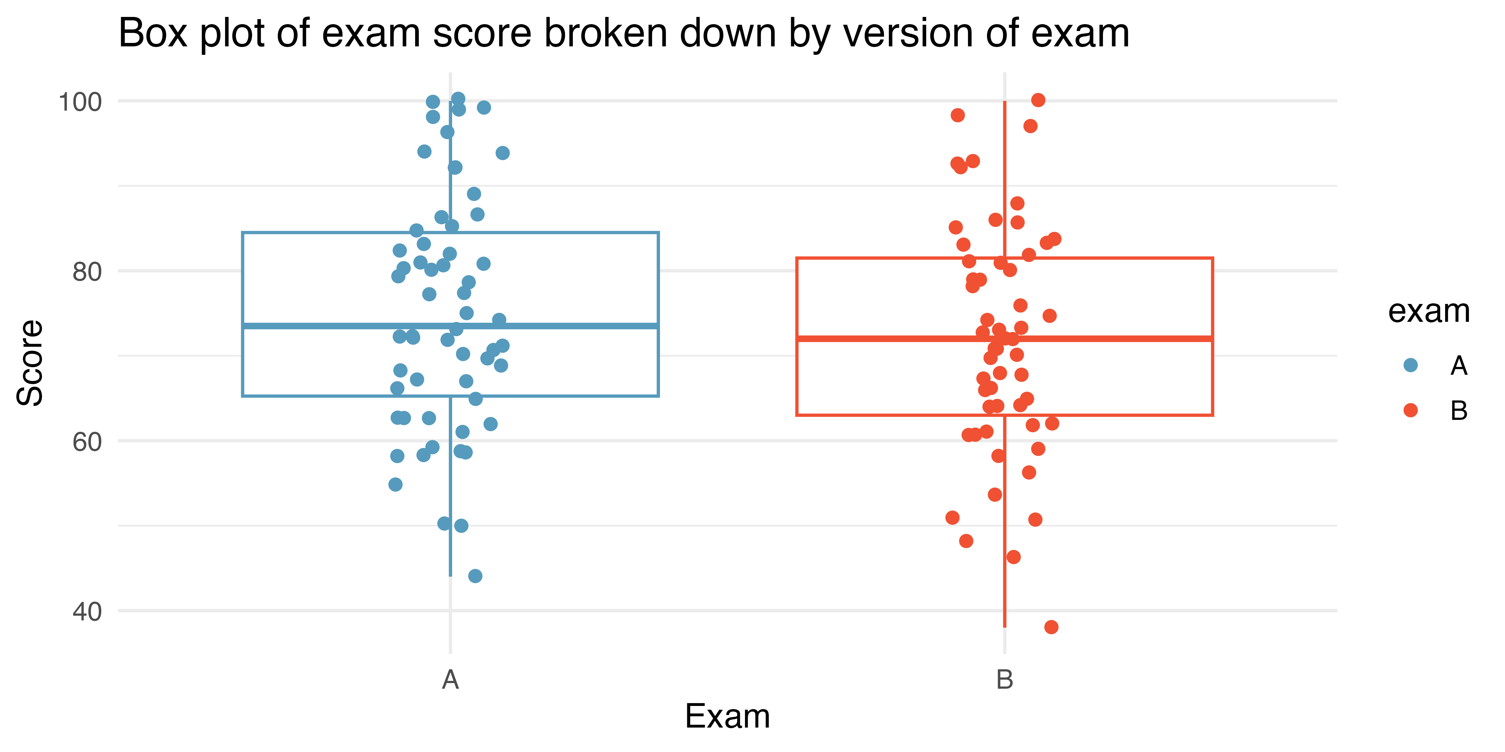
Construct hypotheses to evaluate whether the observed difference in sample means, \(\bar{x}_A - \bar{x}_B=3.1,\) is likely to have happened due to chance, if the null hypothesis is true. We will later evaluate these hypotheses using \(\alpha = 0.01.\)1
Before moving on to evaluate the hypotheses in the previous Guided Practice, let’s think carefully about the dataset. Are the observations across the two groups independent? Are there any concerns about outliers?2
20.1.2 Variability of the statistic
In Chapter 11, the variability of the statistic (previously: \(\hat{p}_1 - \hat{p}_2)\) was visualized after shuffling the observations across the two treatment groups many times. The shuffling process implements the null hypothesis model (that there is no effect of the treatment). In the exam example, the null hypothesis is that exam A and exam B are equally difficult, so the average scores across the two tests should be the same. If the exams were equally difficult, due to natural variability, we would sometimes expect students to do slightly better on exam A \((\bar{x}_A > \bar{x}_B)\) and sometimes expect students to do slightly better on exam B \((\bar{x}_B > \bar{x}_A).\) The question at hand is: does \(\bar{x}_A - \bar{x}_B=3.1\) indicate that exam A is easier than exam B.
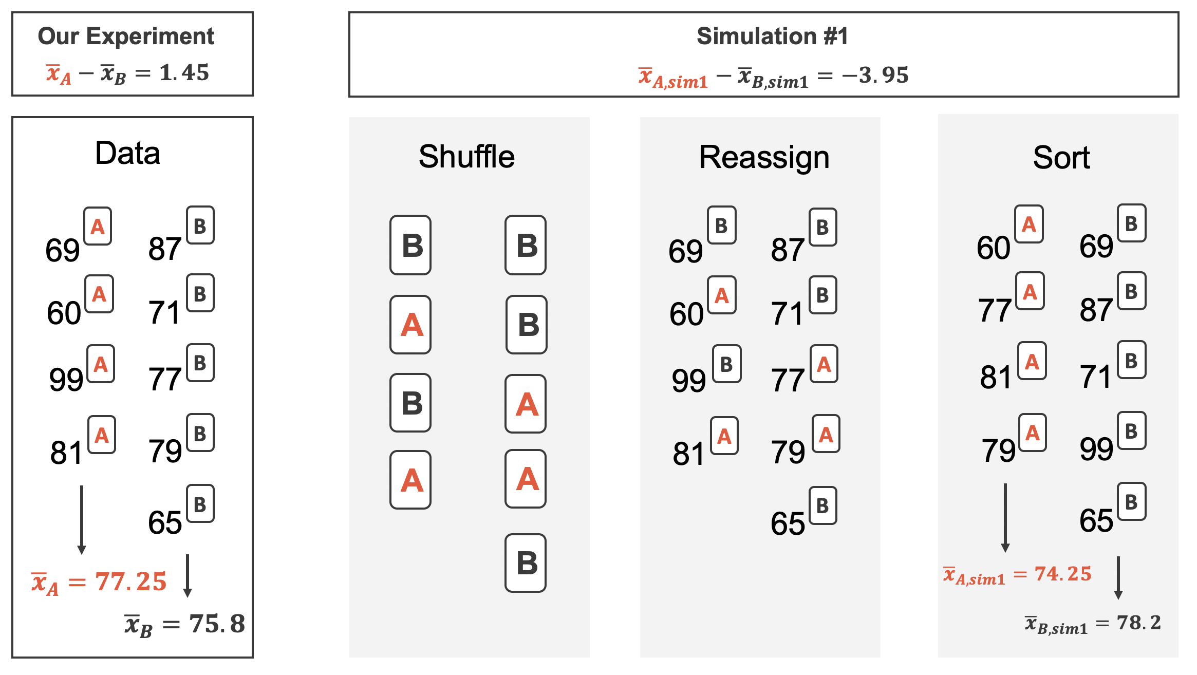
Figure 20.2 shows the process of randomizing the exam to the observed exam scores. If the null hypothesis is true, then the score on each exam should represent the true student ability on that material. It shouldn’t matter whether they were given exam A or exam B. By reallocating which student got which exam, we are able to understand how the difference in average exam scores changes due only to natural variability. There is only one iteration of the randomization process in Figure 20.2, leading to one simulated difference in average scores.
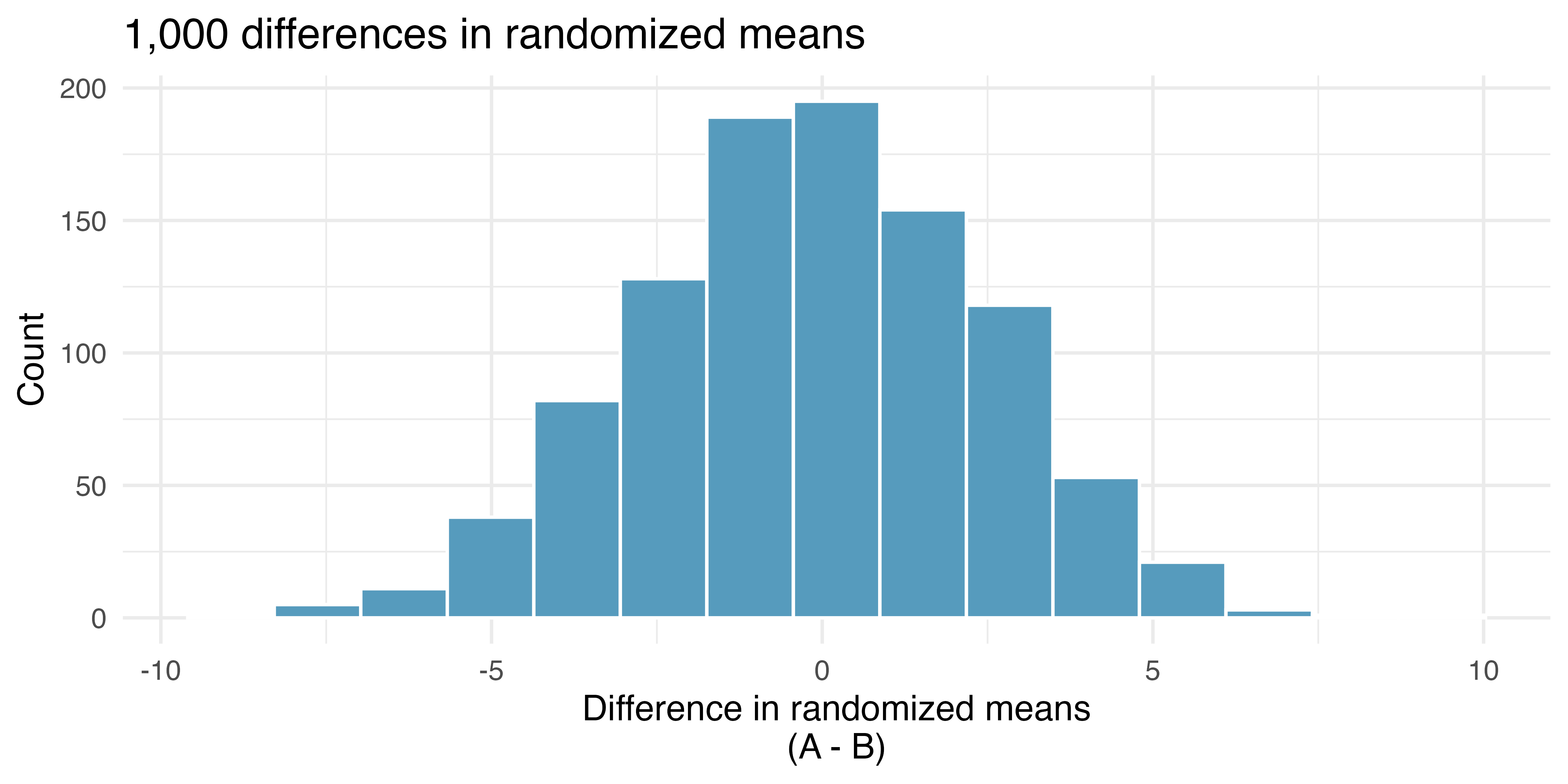
Building on Figure 20.2, Figure 20.3 shows the values of the simulated statistics \(\bar{x}_{1, sim} - \bar{x}_{2, sim}\) over 1,000 random simulations. We see that, just by chance, the difference in scores can range anywhere from -10 points to +10 points.
20.1.3 Observed statistic vs. null statistics
The goal of the randomization test is to assess the observed data, here the statistic of interest is \(\bar{x}_A - \bar{x}_B=3.1.\) The randomization distribution allows us to identify whether a difference of 3.1 points is more than one would expect by natural variability of the scores if the two tests were equally difficult. By plotting the value of 3.1 on Figure 20.4, we can measure how different or similar 3.1 is to the randomized differences which were generated under the null hypothesis.
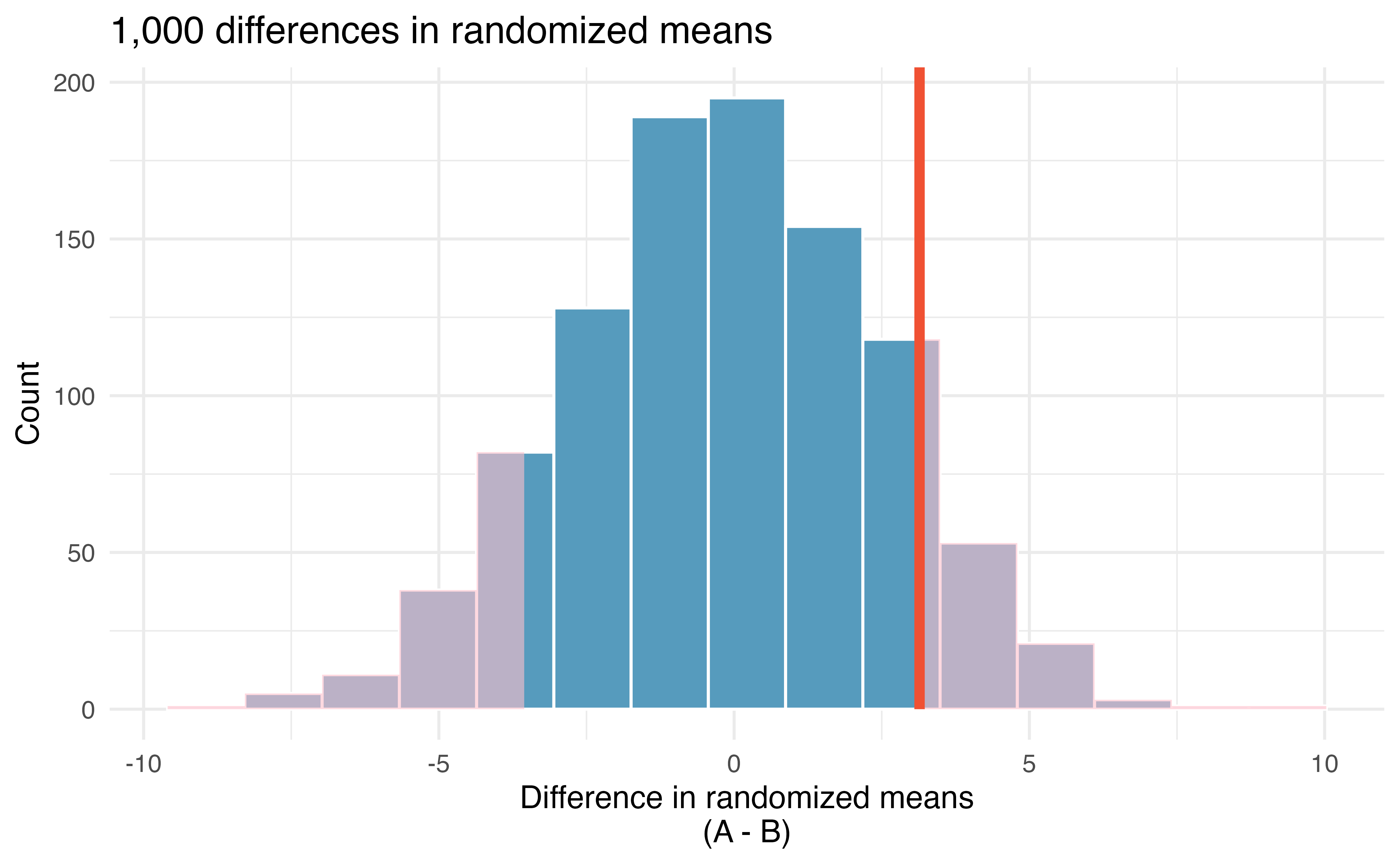
Approximate the p-value depicted in Figure 20.4, and provide a conclusion in the context of the case study.
Using software, we can find the number of shuffled differences in means that are less than the observed difference (of 3.14) is 900 (out of 1,000 randomizations). So 10% of the simulations are larger than the observed difference. To get the p-value, we double the proportion of randomized differences which are larger than the observed difference, p-value = 0.2.
Previously, we specified that we would use \(\alpha = 0.01.\) Since the p-value is larger than \(\alpha,\) we do not reject the null hypothesis. That is, the data do not convincingly show that one exam version is more difficult than the other, and the teacher should not be convinced that they should add points to the Version B exam scores.
The large p-value and consistency of \(\bar{x}_A - \bar{x}_B=3.1\) with the randomized differences leads us to not reject the null hypothesis. Said differently, there is no evidence to think that one of the tests is easier than the other. One might be inclined to conclude that the tests have the same level of difficulty, but that conclusion would be wrong. The hypothesis testing framework is set up only to reject a null claim, it is not set up to validate a null claim. As we concluded, the data are consistent with exams A and B being equally difficult, but the data are also consistent with exam A being 3.1 points “easier” than exam B. The data are not able to adjudicate on whether the exams are equally hard or whether one of them is slightly easier. Indeed, conclusions where the null hypothesis is not rejected often seem unsatisfactory. However, in this case, the teacher and class are probably all relieved that there is no evidence to demonstrate that one of the exams is more difficult than the other.
20.2 Bootstrap confidence interval for the difference in means
Before providing a full example working through a bootstrap analysis on actual data, we return to the fictional Awesome Auto example as a way to visualize the two sample bootstrap setting. Consider an expanded scenario where the research question centers on comparing the average price of a car at one Awesome Auto franchise (Group 1) to the average price of a car at a different Awesome Auto franchise (Group 2). The process of bootstrapping can be applied to each Group separately, and the differences of means recalculated each time. Figure 20.5 visually describes the bootstrap process when interest is in a statistic computed on two separate samples. The analysis proceeds as in the one sample case, but now the (single) statistic of interest is the difference in sample means. That is, a bootstrap resample is done on each of the groups separately, but the results are combined to have a single bootstrapped difference in means. Repetition will produce \(k\) bootstrapped differences in means, and the histogram will describe the natural sampling variability associated with the difference in means.
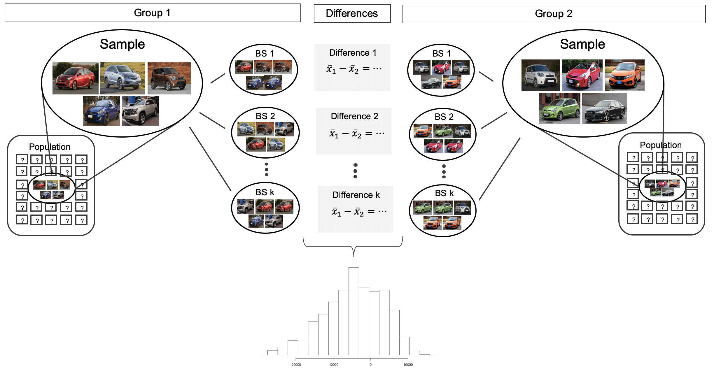
In the following sections, we leave the fictional setting of Awesome Auto and apply the bootstrap method to actual datasets investigating whether embryonic stem cells help improve heart function and later to investigate characteristics of births. Note that the fictional setting allowed us to visualize the bootstrap method because we had samples of size five. The visualization was important in understanding how the bootstrap method works. However, the bootstrap relies heavily on the sample being an outstanding proxy for the population, and five observations are almost never enough to truly represent the nuances of a full population. To that end, we apply bootstrap methods with much larger sample sizes, as seen in the 1000 random samples provided in the births data.
20.2.1 Observed data
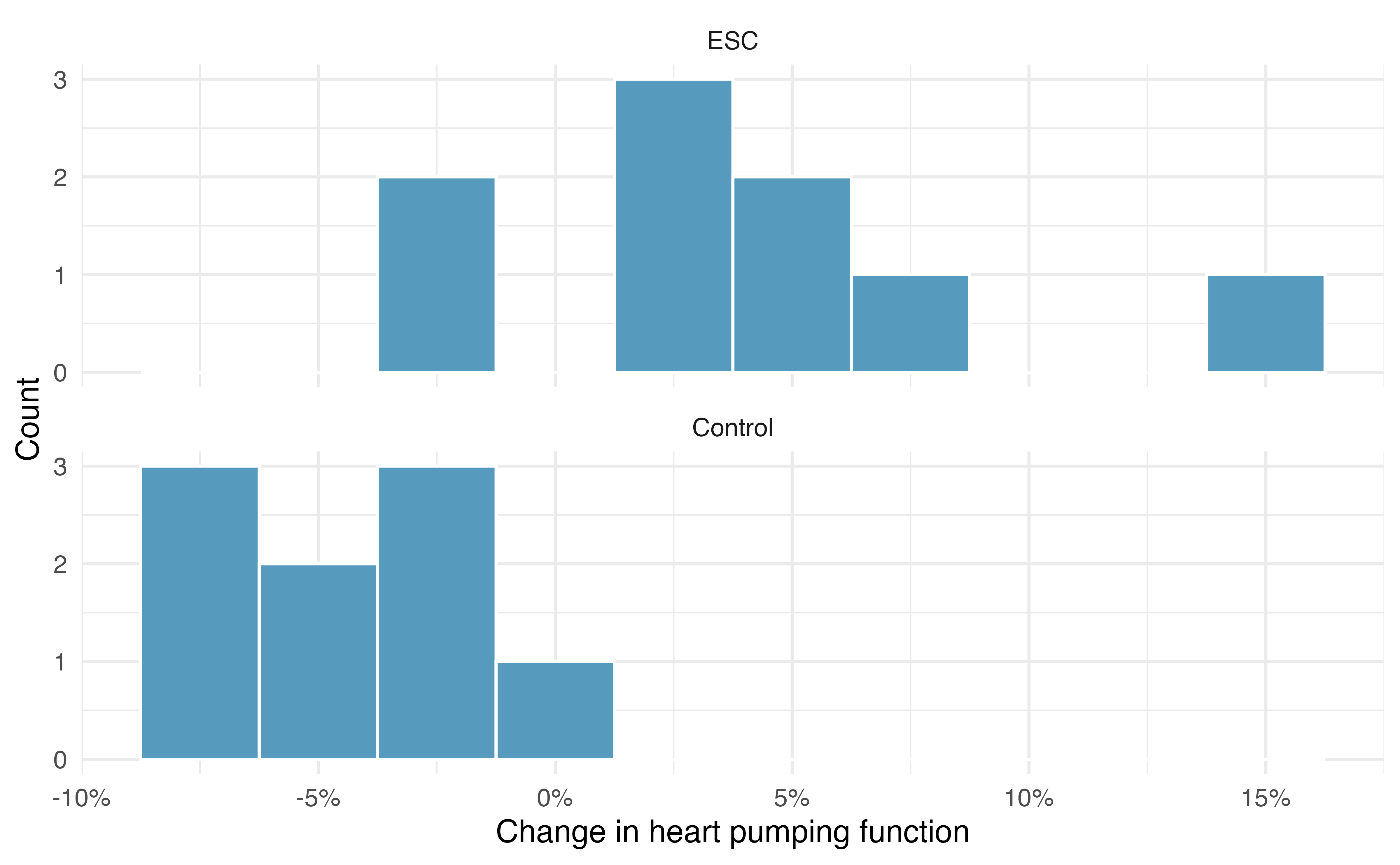
Does treatment using embryonic stem cells (ESCs) help improve heart function following a heart attack? Table 20.2 contains summary statistics for an experiment to test ESCs in sheep that had a heart attack. Each of these sheep was randomly assigned to the ESC or control group, and the change in their hearts’ pumping capacity was measured in the study. (Ménard et al. 2005) Figure 20.8 provides histograms of the two datasets. A positive value corresponds to increased pumping capacity, which generally suggests a stronger recovery. Our goal will be to identify a 95% confidence interval for the effect of ESCs on the change in heart pumping capacity relative to the control group.
| Group | n | Mean | SD |
|---|---|---|---|
| ESC | 9 | 3.50 | 5.17 |
| Control | 9 | -4.33 | 2.76 |
The point estimate of the difference in the heart pumping variable is straightforward to find: it is the difference in the sample means.
\[\bar{x}_{esc} - \bar{x}_{control}\ =\ 3.50 - (-4.33)\ =\ 7.83\]
20.2.2 Variability of the statistic
As we saw in Section 17.2, we will use bootstrapping to estimate the variability associated with the difference in sample means when taking repeated samples. In a method akin to two proportions, a separate sample is taken with replacement from each group (here ESCs and control), the sample means are calculated, and their difference is taken. The entire process is repeated multiple times to produce a bootstrap distribution of the difference in sample means (without the null hypothesis assumption).
Figure 20.6 displays the variability of the differences in means with the 90% percentile and SE confidence intevals super imposed.
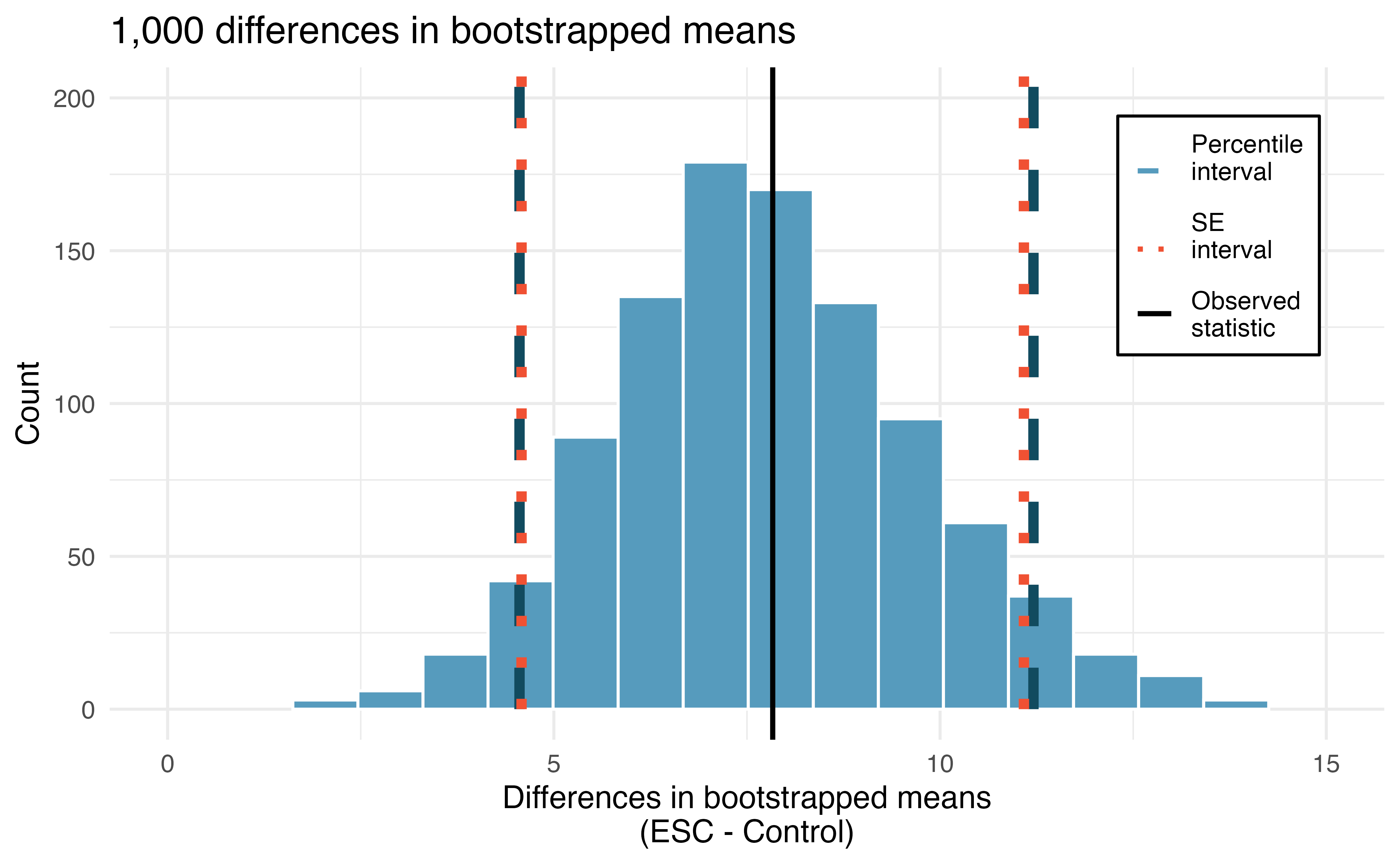
Using the histogram of bootstrapped difference in means, estimate the standard error of the differences in sample means, \(\bar{x}_{ESC} - \bar{x}_{Control}.\)3
Choose one of the bootstrap confidence intervals for the true difference in average pumping capacity, \(\mu_{ESC} - \mu_{Control}.\) Does the interval show that there is a difference across the two treatments?
Because neither of the 90% intervals (either percentile or SE) above overlap zero (note that zero is never one of the bootstrapped differences so 95% and 99% intervals would have given the same conclusion!), we conclude that the ESC treatment is substantially better with respect to heart pumping capacity than the control.
Because the study is a randomized controlled experiment, we can conclude that it is the treatment (ESC) which is causing the change in pumping capacity.
20.3 Mathematical model for testing the difference in means
Every year, the US releases to the public a large dataset containing information on births recorded in the country. This dataset has been of interest to medical researchers who are studying the relation between habits and practices of expectant mothers and the birth of their children. We will work with a random sample of 1,000 cases from the dataset released in 2014.
20.3.1 Observed data
Four cases from this dataset are represented in Table 20.3. We are particularly interested in two variables: weight and smoke. The weight variable represents the weights of the newborns and the smoke variable describes which mothers smoked during pregnancy.
births14 dataset. The empty cells indicate missing data.
| fage | mage | weeks | visits | gained | weight | sex | habit |
|---|---|---|---|---|---|---|---|
| 34 | 34 | 37 | 14 | 28 | 6.96 | male | nonsmoker |
| 36 | 31 | 41 | 12 | 41 | 8.86 | female | nonsmoker |
| 37 | 36 | 37 | 10 | 28 | 7.51 | female | nonsmoker |
| 16 | 38 | 29 | 6.19 | male | nonsmoker |
We would like to know, is there convincing evidence that newborns from mothers who smoke have a different average birth weight than newborns from mothers who do not smoke? We will use data from this sample to try to answer this question.
Set up appropriate hypotheses to evaluate whether there is a relationship between a mother smoking and average birth weight.
The null hypothesis represents the case of no difference between the groups.
- \(H_0:\) There is no difference in average birth weight for newborns from mothers who did and did not smoke. In statistical notation: \(\mu_{n} - \mu_{s} = 0,\) where \(\mu_{n}\) represents non-smoking mothers and \(\mu_s\) represents mothers who smoked.
- \(H_A:\) There is some difference in average newborn weights from mothers who did and did not smoke \((\mu_{n} - \mu_{s} \neq 0).\)
Table 20.4 displays sample statistics from the data. We can see that the average birth weight of babies born to smoker moms is lower than those born to nonsmoker moms.
births14 dataset.
| Habit | n | Mean | SD |
|---|---|---|---|
| nonsmoker | 867 | 7.27 | 1.23 |
| smoker | 114 | 6.68 | 1.60 |
20.3.2 Variability of the statistic
We check the two conditions necessary to model the difference in sample means using the \(t\)-distribution.
- Because the data come from a simple random sample, the observations are independent, both within and between samples.
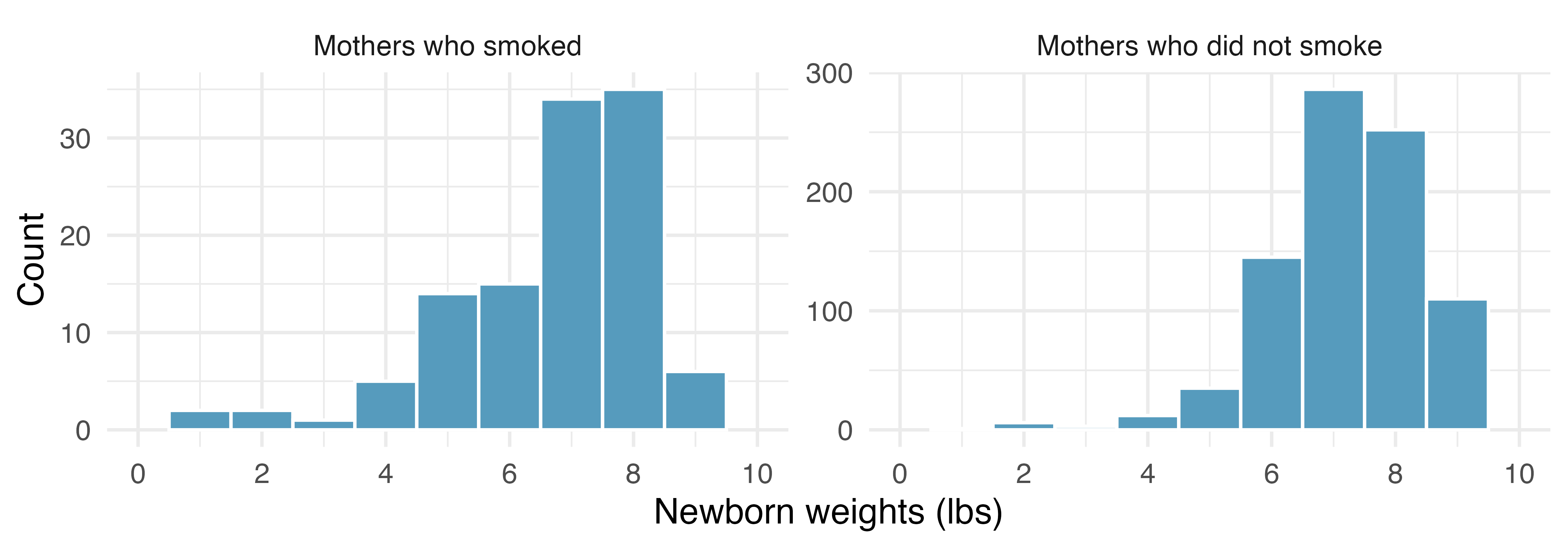
- With both groups over 30 observations, we inspect the data in Figure 20.7 for any particularly extreme outliers and find none.
Since both conditions are satisfied, the difference in sample means may be modeled using a \(t\)-distribution.
The summary statistics in Table 20.4 may be useful for this Guided Practice. What is the point estimate of the population difference, \(\mu_{n} - \mu_{s}\)?4
20.3.3 Observed statistic vs. null statistics
The test statistic for comparing two means is a T.
The T score is a ratio of how the groups differ as compared to how the observations within a group vary.
\[T = \frac{(\bar{x}_1 - \bar{x}_2) - 0}{\sqrt{s_1^2/n_1 + s_2^2/n_2}}\]
When the null hypothesis is true and the conditions are met, T has a t-distribution with \(df = min(n_1 - 1, n_2 -1).\)
Conditions:
- Independent observations within and between groups.
- Large samples and no extreme outliers.
Compute the standard error of the point estimate for the average difference between the weights of babies born to nonsmoker and smoker mothers.5
Complete the hypothesis test started in the previous Example and Guided Practice on births14 dataset and research question. Use a discernibility level of \(\alpha=0.05.\) For reference, \(\bar{x}_{n} - \bar{x}_{s} = 0.59,\) \(SE = 0.16,\) and the sample sizes were \(n_n = 867\) and \(n_s = 114.\)
We can find the test statistic for this test using the previous information:
\[T = \frac{\ 0.59 - 0\ }{0.16} = 3.69\]
We find the single tail area using software. We’ll use the smaller of \(n_n - 1 = 866\) and \(n_s - 1 = 113\) as the degrees of freedom: \(df = 113.\) The one tail area is roughly 0.00017; doubling this value gives the two-tail area and p-value, 0.00034.
The p-value is smaller than the discernibility level, 0.05, so we reject the null hypothesis. The data provide statistically discernible evidence of a difference in the average weights of babies born to mothers who smoked during pregnancy and those who did not.
This result is likely not surprising. We all know that smoking is bad for you and you’ve probably also heard that smoking during pregnancy is not just bad for the mother but also for the baby as well. In fact, some in the tobacco industry actually had the audacity to tout that as a benefit of smoking:
It’s true. The babies born from women who smoke are smaller, but they’re just as healthy as the babies born from women who do not smoke. And some women would prefer having smaller babies. - Joseph Cullman, Philip Morris’ Chairman of the Board on CBS’ Face the Nation, Jan 3, 1971
Furthermore, health differences between babies born to mothers who smoke and those who do not are not limited to weight differences.6
A small note on the power of the independent t-test (recall the discussion of power in Section 14.4). It turns out that the independent t-test given here is often less powerful than the paired t-test discussed in Section 21.3. That said, depending on how the data are collected, we don’t always have a mechanism for pairing the data and reducing the inherent variability across observations.
20.4 Mathematical model for estimating the difference in means
20.4.1 Observed data
As with hypothesis testing, for the question of whether we can model the difference using a \(t\)-distribution, we’ll need to check new conditions. Like the 2-proportion cases, we will require a more robust version of independence so we are confident the two groups are also independent. Secondly, we also check for normality in each group separately, which in practice is a check for outliers.
Using the \(t\)-distribution for a difference in means.
The \(t\)-distribution can be used for inference when working with the standardized difference of two means if
- Independence (extended). The data are independent within and between the two groups, e.g., the data come from independent random samples or from a randomized experiment.
- Normality. We check the outliers for each group separately.
The standard error may be computed as
\[SE = \sqrt{\frac{\sigma_1^2}{n_1} + \frac{\sigma_2^2}{n_2}}\]
The official formula for the degrees of freedom is quite complex and is generally computed using software, so instead you may use the smaller of \(n_1 - 1\) and \(n_2 - 1\) for the degrees of freedom if software isn’t readily available.
Recall that the margin of error is defined by the standard error. The margin of error for \(\bar{x}_1 - \bar{x}_2\) can be directly obtained from \(SE(\bar{x}_1 - \bar{x}_2).\)
Margin of error for \(\bar{x}_1 - \bar{x}_2.\)
The margin of error is \(t^\star_{df} \times \sqrt{\frac{s_1^2}{n_1} + \frac{s_2^2}{n_2}}\) where \(t^\star_{df}\) is calculated from a specified percentile on the t-distribution with df degrees of freedom.
20.4.2 Variability of the statistic
Can the \(t\)-distribution be used to make inference using the point estimate, \(\bar{x}_{esc} - \bar{x}_{control} = 7.83\)?
First, we check for independence. Because the sheep were randomized into the groups, independence within and between groups is satisfied.
Figure 20.8 does not reveal any clear outliers in either group. (The ESC group does look a bit more variable, but this is not the same as having clear outliers.)
With both conditions met, we can use the \(t\)-distribution to model the difference of sample means.
Generally, we use statistical software to find the appropriate degrees of freedom, or if software isn’t available, we can use the smaller of \(n_1 - 1\) and \(n_2 - 1\) for the degrees of freedom, e.g., if using a \(t\)-table to find tail areas. For transparency in the Examples and Guided Practice, we’ll use the latter approach for finding \(df\); in the case of the ESC example, this means we’ll use \(df = 8.\)
Calculate a 95% confidence interval for the effect of ESCs on the change in heart pumping capacity of sheep after they’ve suffered a heart attack.
We will use the sample difference and the standard error that we computed earlier:
\[ \begin{aligned} \bar{x}_{esc} - \bar{x}_{control} &= 7.83 \\ SE &= \sqrt{\frac{5.17^2}{9} + \frac{2.76^2}{9}} = 1.95 \end{aligned} \]
Using \(df = 8,\) we can identify the critical value of \(t^{\star}_{8} = 2.31\) for a 95% confidence interval. Finally, we can enter the values into the confidence interval formula:
\[ \begin{aligned} \text{point estimate} \ &\pm\ t^{\star} \times SE \\ 7.83 \ &\pm\ 2.31\times 1.95 \\ (3.32 \ &, \ 12.34) \end{aligned} \]
We are 95% confident that the heart pumping function in sheep that received embryonic stem cells is between 3.32% and 12.34% higher than for sheep that did not receive the stem cell treatment.
20.5 Chapter review
20.5.1 Summary
In this chapter we extended the single mean inferential methods to questions of differences in means. You may have seen parallels from the chapters that extended a single proportion (Chapter 16) to differences in proportions (Chapter 17). When considering differences in sample means (indeed, when considering many quantitative statistics), we use the t-distribution to describe the sampling distribution of the T score (the standardized difference in sample means). Ideas of confidence level and type of error which might occur from a hypothesis test conclusion are similar to those seen in other chapters (see Chapter 14).
20.5.2 Terms
The terms introduced in this chapter are presented in Table 20.5. If you’re not sure what some of these terms mean, we recommend you go back in the text and review their definitions. You should be able to easily spot them as bolded text.
| difference in means | SE difference in means | t-CI |
| point estimate | T score | t-test |
20.6 Exercises
Answers to odd-numbered exercises can be found in Appendix A.20.
-
Experimental baker. A baker working on perfecting their bagel recipe is experimenting with active dry (AD) and instant (I) yeast. They bake a dozen bagels with each type of yeast and score each bagel on a scale of 1 to 10 on how well the bagels rise. They come up with the following set of hypotheses for evaluating whether there is a difference in the average rise of bagels baked with active dry and instant yeast. What is wrong with the hypotheses as stated?
\[H_0: \bar{x}_{AD} \leq \bar{x}_{I} \quad \quad H_A: \bar{x}_{AD} > \bar{x}_{I}\]
- Fill in the blanks. We use a ___ to evaluate if data provide convincing evidence of a difference between two population means and we use a ___ to estimate this difference.
-
Diamonds, randomization test. The prices of diamonds go up as the carat weight increases, but the increase is not smooth. For example, the difference between the size of a 0.99 carat diamond and a 1 carat diamond is undetectable to the naked human eye, but the price of a 1 carat diamond tends to be much higher than the price of a 0.99 carat diamond. We have two random samples of diamonds: 23 0.99 carat diamonds and 23 1 carat diamonds. In order to be able to compare equivalent units, we first divide the price for each diamond by 100 times its weight in carats. That is, for a 0.99 carat diamond, we divide the price by 99 and for a 1 carat diamond, we divide it by 100. Then, we randomize the carat weight to the price values in order simulate the null distribution of differences in average prices of 0.99 carat and 1 carat diamonds. The null distribution (with 1,000 randomized differences) is shown below and depicts the distribution of differences in sample means (of price per carat) if there really was no difference in the population from which these diamonds came.7 (Wickham 2016)
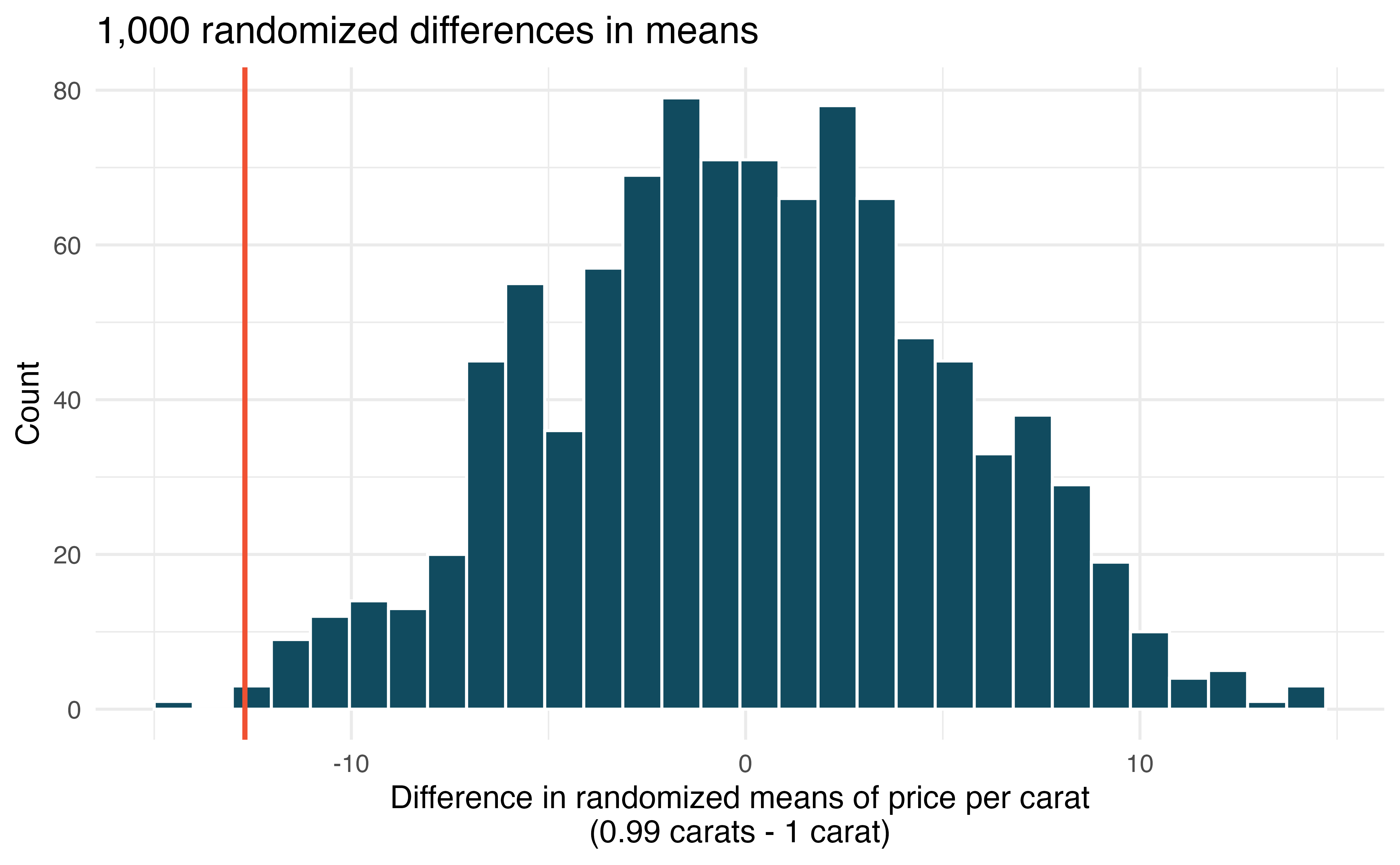
Using the randomization distribution, conduct a hypothesis test to evaluate if there is a difference between the prices per carat of diamonds that weigh 0.99 carats and diamonds that weigh 1 carat. Make sure to state your hypotheses clearly and interpret your results in context of the data. (Wickham 2016)
-
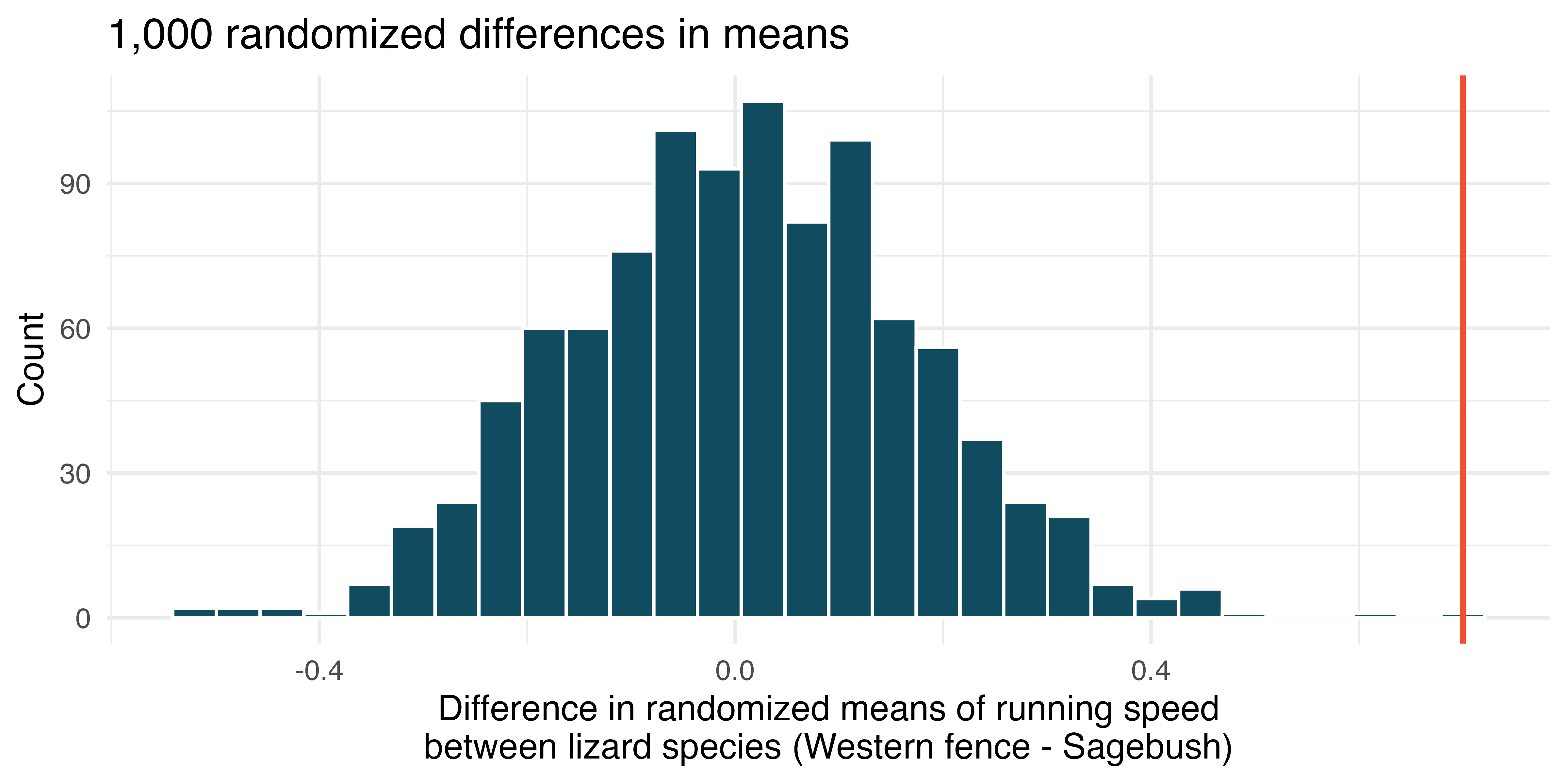
Lizards running, randomization test. In order to assess physiological characteristics of common lizards, data on top speeds (in m/sec) measured on a laboratory race track for two species of lizards: Western fence lizard (Sceloporus occidentalis) and Sagebrush lizard (Sceloporus graciosus). The original observed difference in lizard speeds is \(\bar{x}_{Western fence} - \bar{x}_{Sagebrush} = 0.7 \mbox{m/sec}.\) The histogram below shows the distribution of average differences when speed has been randomly allocated across lizard species 1,000 times. Using the randomization distribution, conduct a hypothesis test to evaluate if there is a difference between the average speed of the Western fence lizard as compared to the Sagebrush lizard. Make sure to state your hypotheses clearly and interpret your results in context of the data.8 (Adolph 1987)
-
Diamonds, bootstrap interval. We have data on two random samples of diamonds: 23 0.99 carat diamonds and 23 1 carat diamonds. Provided below is a histogram of bootstrap differences in means of price per carat of diamonds that weigh 0.99 carats and diamonds that weigh 1 carat. (Wickham 2016)
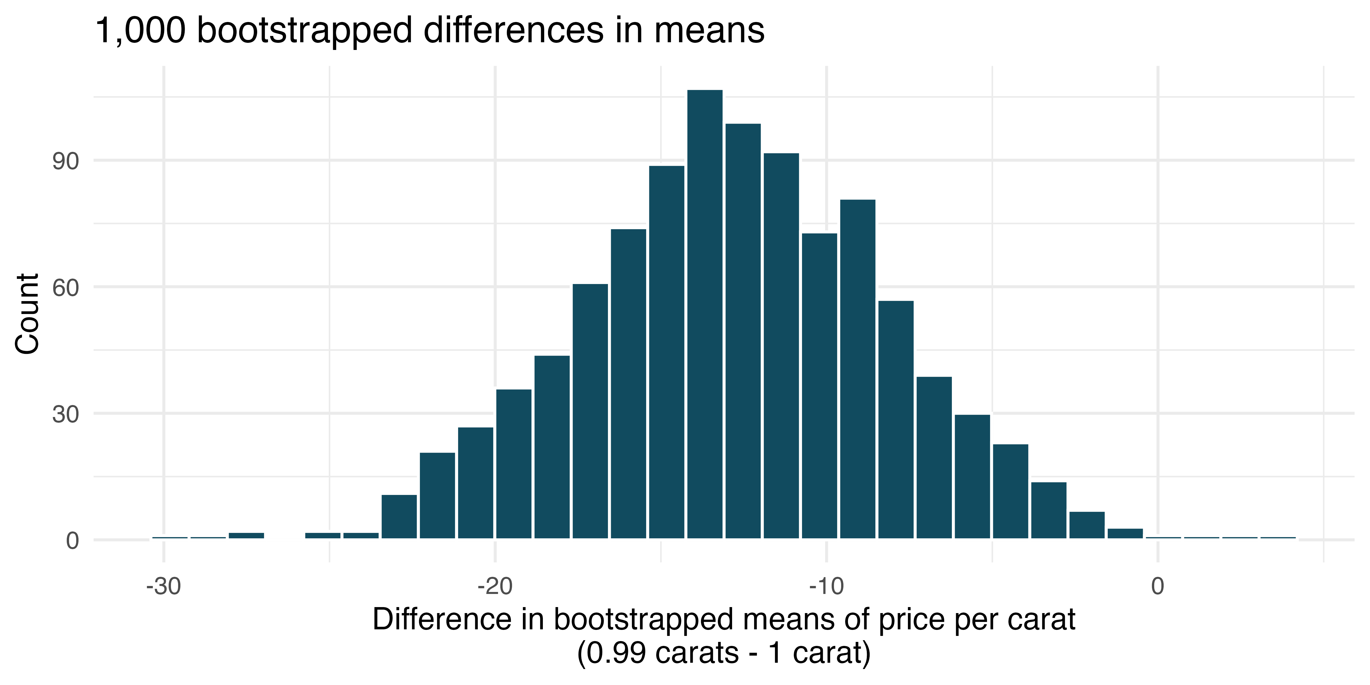
Using the bootstrap distribution, create a (rough) 95% bootstrap percentile confidence interval for the true population difference in prices per carat of diamonds that weigh 0.99 carats and 1 carat.
Using the bootstrap distribution, create a (rough) 95% bootstrap SE confidence interval for the true population difference in prices per carat of diamonds that weigh 0.99 carats and 1 carat. Note that the standard error of the bootstrap distribution is 4.64.
-
Lizards running, bootstrap interval. We have data on top speeds (in m/sec) measured on a laboratory race track for two species of lizards: Western fence lizard (Sceloporus occidentalis) and Sagebrush lizard (Sceloporus graciosus). The bootstrap distribution below describes the variability of difference in means captured from 1,000 bootstrap samples of the lizard data. (Adolph 1987)
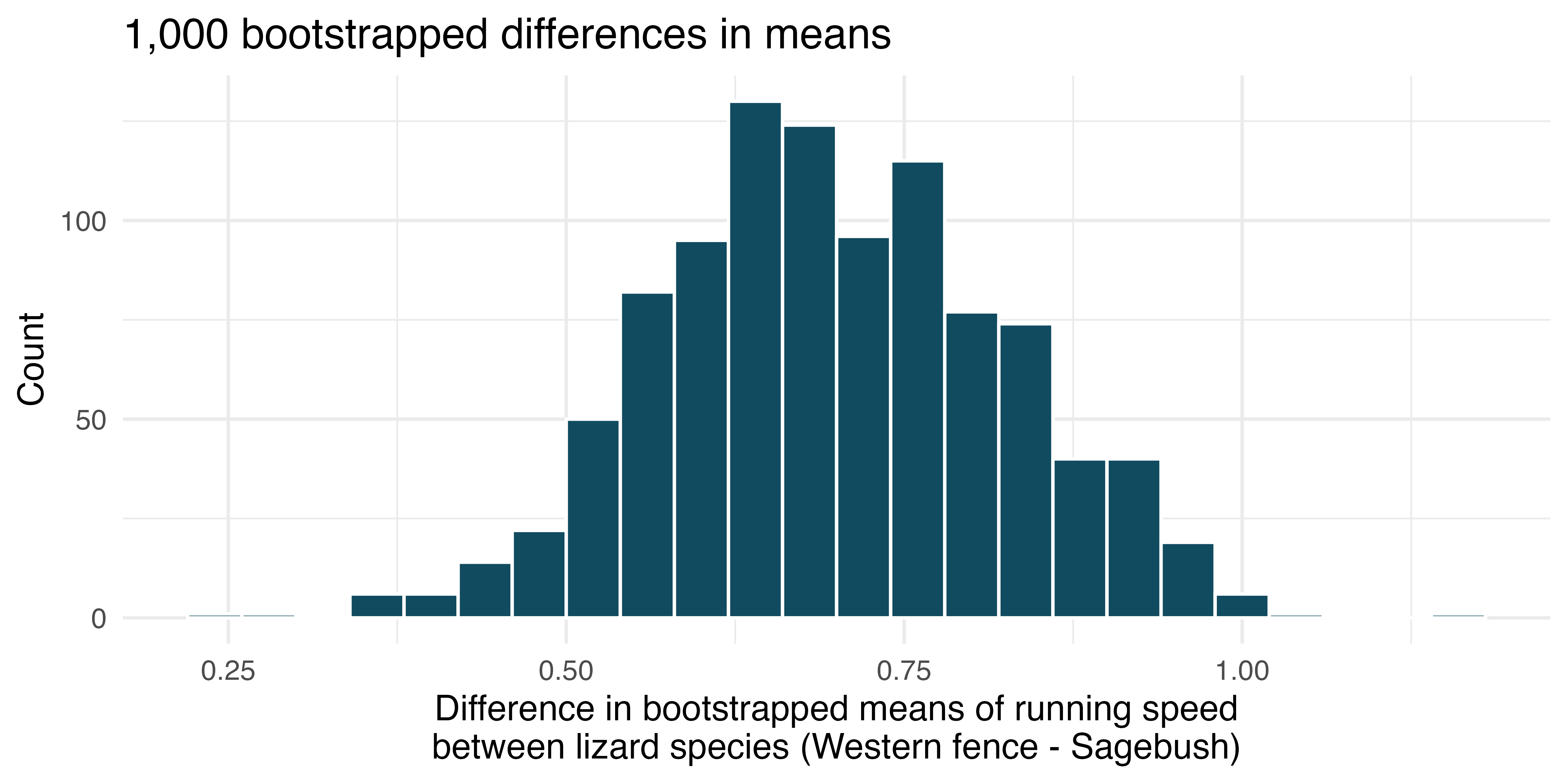
Using the bootstrap distribution, create a (rough) 90% percentile bootrap confidence interval for the true population difference in average speed of the Western fence lizard as compared with Sagebrush lizard.
Using the bootstrap distribution, create a (rough) 90% bootstrap SE confidence interval for the true population difference in average speed of the Western fence lizard as compared with Sagebrush lizard.
- Weight loss. You are reading an article in which the researchers have created a 95% confidence interval for the difference in average weight loss for two diets. They are 95% confident that the true difference in average weight loss over 6 months for the two diets is somewhere between (1 lb, 25 lbs). The authors claim that, “therefore diet A (\(\bar{x}_A\) = 20 lbs average loss) results in a much larger average weight loss as compared to diet B (\(\bar{x}_B\) = 7 lbs average loss).” Comment on the authors’ claim.
-
Possible randomized means. Data were collected on data from two groups (A and B). There were 3 measurements taken on Group A and two measurements in Group B.
Group Measurement 1 Measurement 2 Measurement 3 A 1 15 5 B 7 3 If the data are (repeatedly) randomly allocated across the two conditions, provide the following: (1) the values which are assigned to group A, (2) the values which are assigned to group B, and (3) the difference in averages \((\bar{x}_A - \bar{x}_B)\) for each of the following:
When the randomized difference in averages is as large as possible.
When the randomized difference in averages is as small as possible (a big in magnitude negative number).
When the randomized difference in averages is as close to zero as possible.
When the observed values are randomly assigned to the two groups, to which of the previous parts would you expect the difference in means to fall closest? Explain your reasoning.
-
Diamonds, mathematical test. We have data on two random samples of diamonds: one with diamonds that weigh 0.99 carats and one with diamonds that weigh 1 carat. Each sample has 23 diamonds. Sample statistics for the price per carat of diamonds in each sample are provided below. Conduct a hypothesis test using a mathematical model to evaluate if there is a difference between the prices per carat of diamonds that weigh 0.99 carats and diamonds that weigh 1 carat Make sure to state your hypotheses clearly, check relevant conditions, and interpret your results in context of the data. (Wickham 2016)
Mean SD n 0.99 carats $44.51 $13.32 23 1 carat $57.20 $18.19 23 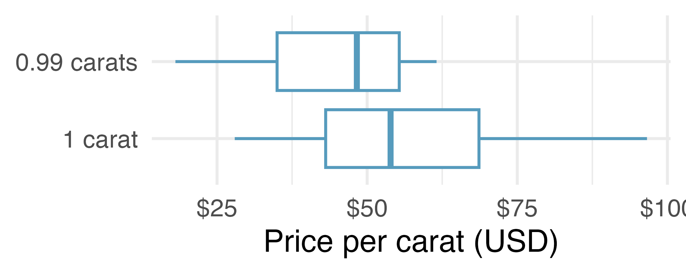
A/B testing. A/B testing is a user experience research methodology where two variants of a page are shown to users at random. A company wants to evaluate whether users will spend more time, on average, on Page A or Page B using an A/B test. Two user experience designers at the company, Lucie and Müge, are tasked with conducting the analysis of the data collected. They agree on how the null hypothesis should be set: on average, users spend the same amount of time on Page A and Page B. Lucie believes that Page B will provide a better experience for users and hence wants to use a one-tailed test, Müge believes that a two-tailed test would be a better choice. Which designer do you agree with, and why?
-
Diamonds, mathematical interval. We have data on two random samples of diamonds: one with diamonds that weigh 0.99 carats and one with diamonds that weigh 1 carat. Each sample has 23 diamonds. Sample statistics for the price per carat of diamonds in each sample are provided below. Assuming that the conditions for conducting inference using a mathematical model are satisfied, construct a 95% confidence interval for the true population difference in prices per carat of diamonds that weigh 0.99 carats and 1 carat. (Wickham 2016)
Mean SD n 0.99 carats $44.51 $13.32 23 1 carat $57.20 $18.19 23
-
True / False: comparing means. Determine if the following statements are true or false, and explain your reasoning for statements you identify as false.
As the degrees of freedom increases, the \(t\)-distribution approaches normality.
If a 95% confidence interval for the difference between two population means contains 0, a 99% confidence interval calculated based on the same two samples will also contain 0.
If a 95% confidence interval for the difference between two population means contains 0, a 90% confidence interval calculated based on the same two samples will also contain 0.
-
Difference of means. We collect two random samples from two different populations In each part below, consider the sample means \(\bar{x}_1\) and \(\bar{x}_2\) that we might observe from these two samples.
Mean Standard deviation Sample size Population 1 15 20 50 Population 2 20 10 30 What is the associated mean and standard deviation of \(\bar{x}_1\)?
What is the associated mean and standard deviation of \(\bar{x}_2\)?
Calculate and interpret the mean and standard deviation associated with the difference in sample means for the two groups, \(\bar{x}_2 - \bar{x}_1\).
How are the standard deviations from parts (a), (b), and (c) related?
- Mindfulness intervention for nurses. In order to address extremely challenging and stressful situations for intensive care unit nurses, researchers ran a mindfulness-based intervention (MBI) study on 60 nurses working in three hospitals in El-Beheira, Egypt. The participants were randomly allocated to one of the two groups: the treatment group (MBI) received 8 MBI sessions and the control group received no intervention. The nurses’ emotional exhaustion was measured using 9 items from a questionnaire of the Maslach Burnout Inventory-Human Services Survey for Medical Personnel; the questions are recorded on a Likert scale where 0 indicated “Never” and 6 indicates “Every day”. Nurses in the treatment group had an emotional exhaustion score of 15.47, with a standard deviation of 4.44, and nurses in the control group had an emotional exhaustion score of 32.43, with a standard deviation of 8.87. Do these data provide convincing evidence that the emotional exhaustion decrease is different for the patients in the treatment group compared to the control group? Assume that conditions for conducting inference using mathematical models are satisfied. (Othman et al. 2023)
-
Chicken diet: horsebean vs. linseed. Chicken farming is a multi-billion dollar industry, and any methods that increase the growth rate of young chicks can reduce consumer costs while increasing company profits, possibly by millions of dollars. An experiment was conducted to measure and compare the effectiveness of various feed supplements on the growth rate of chickens. Newly hatched chicks were randomly allocated into six groups, and each group was given a different feed supplement. In this exercise we consider chicks that were fed horsebean and linseed. Below are some summary statistics from this dataset along with box plots showing the distribution of weights by feed type.9 (McNeil 1977)
Horsebean Linseed Mean 160.2 218.8 SD 38.6 52.2 n 10.0 12.0 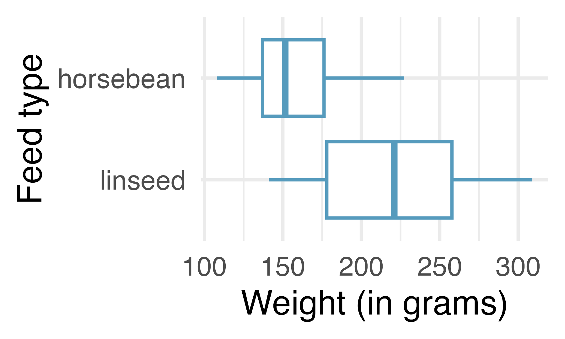
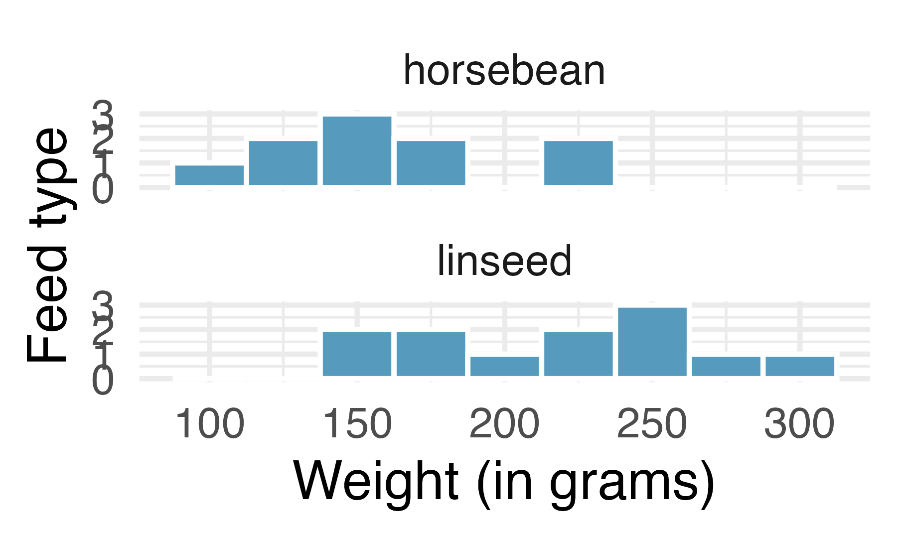
Describe the distributions of weights of chickens that were fed horsebean and linseed.
Do these data provide strong evidence that the average weights of chickens that were fed linseed and horsebean are different? Use a 5% discernibility level.
What type of error might we have committed? Explain.
Would your conclusion change if we used \(\alpha = 0.01\)?
-
Fuel efficiency in the city. Each year the US Environmental Protection Agency (EPA) releases fuel economy data on cars manufactured in that year. Below are summary statistics on fuel efficiency (in miles/gallon) from random samples of cars with manual and automatic transmissions manufactured in 2021. Do these data provide strong evidence of a difference between the average fuel efficiency of cars with manual and automatic transmissions in terms of their average city mileage?10 (US DOE EPA 2021)
CITY Mean SD n Automatic 17.4 3.44 25 Manual 22.7 4.58 25 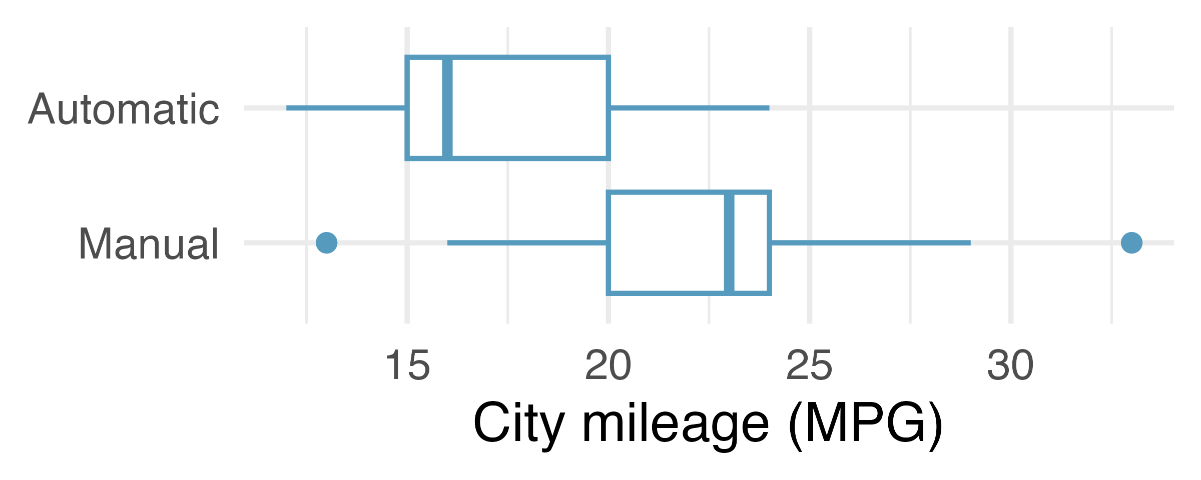
-
Chicken diet: casein vs. soybean. Casein is a common weight gain supplement for humans. Does it have an effect on chickens? An experiment was conducted to measure and compare the effectiveness of various feed supplements on the growth rate of chickens. Newly hatched chicks were randomly allocated into six groups, and each group was given a different feed supplement. In this exercise we consider chicks that were fed casein and soybean. Assume that the conditions for conducting inference using mathematical models are met, and using the data provided below, test the hypothesis that the average weight of chickens that were fed casein is different than the average weight of chickens that were fed soybean. If your hypothesis test yields a statistically discernible result, discuss whether the higher average weight of chickens can be attributed to the casein diet. (McNeil 1977)
Feed type Mean SD n casein 323.58 64.43 12 soybean 246.43 54.13 14
-
Fuel efficiency on the highway. Each year the US Environmental Protection Agency (EPA) releases fuel economy data on cars manufactured in that year. Below are summary statistics on fuel efficiency (in miles/gallon) from random samples of cars with manual and automatic transmissions manufactured in 2021. Do these data provide strong evidence of a difference between the average fuel efficiency of cars with manual and automatic transmissions in terms of their average highway mileage? (US DOE EPA 2021)
HIGHWAY Mean SD n Automatic 23.7 3.90 25 Manual 30.9 5.13 25 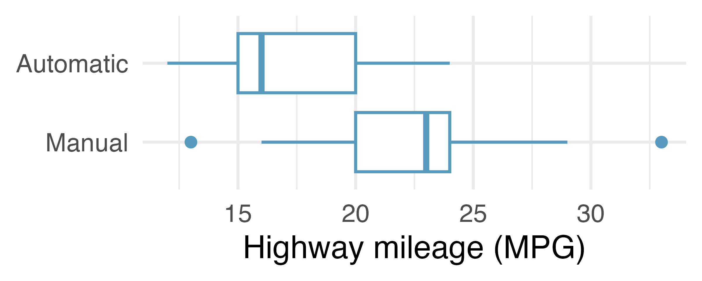
- Gaming, distracted eating, and intake. A group of researchers who are interested in the possible effects of distracting stimuli during eating, such as an increase or decrease in the amount of food consumption, monitored food intake for a group of 44 patients who were randomized into two equal groups. The treatment group ate lunch while playing solitaire, and the control group ate lunch without any added distractions. Patients in the treatment group ate 52.1 grams of biscuits, with a standard deviation of 45.1 grams, and patients in the control group ate 27.1 grams of biscuits, with a standard deviation of 26.4 grams. Do these data provide convincing evidence that the average food intake (measured in amount of biscuits consumed) is different for the patients in the treatment group compared to the control group? Assume that conditions for conducting inference using mathematical models are satisfied. (Oldham-Cooper et al. 2011)
- Gaming, distracted eating, and recall. A group of researchers who are interested in the possible effects of distracting stimuli during eating, such as an increase or decrease in the amount of food consumption, monitored food intake for a group of 44 patients who were randomized into two equal groups. The 22 patients in the treatment group who ate their lunch while playing solitaire were asked to do a serial-order recall of the food lunch items they ate. The average number of items recalled by the patients in this group was 4. 9, with a standard deviation of 1.8. The average number of items recalled by the patients in the control group (no distraction) was 6.1, with a standard deviation of 1.8. Do these data provide strong evidence that the average numbers of food items recalled by the patients in the treatment and control groups are different? Assume that conditions for conducting inference using mathematical models are satisfied. (Oldham-Cooper et al. 2011)
\(H_0:\) the exams are equally difficult, on average. \(\mu_A - \mu_B = 0.\) \(H_A:\) one exam was more difficult than the other, on average. \(\mu_A - \mu_B \neq 0.\)↩︎
Since the exams were shuffled, the “treatment” in this case was randomly assigned, so independence within and between groups is satisfied. The summary statistics suggest the data are roughly symmetric about the mean, and the min/max values do not suggest any outliers of concern.↩︎
The point estimate of the population difference (\(\bar{x}_{ESC} - \bar{x}_{Control}\)) is 7.83.↩︎
The point estimate of the population difference (\(\bar{x}_{n} - \bar{x}_{s}\)) is 0.59.↩︎
\(SE(\bar{x}_{n} - \bar{x}_{s}) = \sqrt{s^2_{n}/ n_{n} + s^2_{s}/n_{s}} = \sqrt{1.23^2/867 + 1.60^2/114} = 0.16\)↩︎
You can watch an episode of John Oliver on Last Week Tonight to explore the present day offenses of the tobacco industry. Please be aware that there is some adult language.↩︎
The
diamondsdata used in this exercise can be found in the ggplot2 R package.↩︎The
lizard_rundata used in this exercise can be found in the openintro R package.↩︎The
chickwtsdata used in this exercise can be found in the datasets R package.↩︎The
epa2021data used in this exercise can be found in the openintro R package.↩︎