22 Inference for comparing many means
In Chapter 20 analysis was done to compare the average population value across two different groups. An important aspect of the analysis was to look at the difference in sample means as an estimate for the difference in population means. When comparing more than two groups, the difference (i.e., subtraction) will not fully capture the nuance in variation across the three or more groups. As with two groups, the research question will focus on whether the group membership is independent of the numerical response variable. Here, independence across groups means that knowledge of the observations in one group does not change what we would expect to happen in the other group. But what happens if the groups are dependent? In this section we focus on a new statistic which incorporates differences in means across more than two groups. Although the ideas in this chapter are quite similar to the t-test, they have earned themselves their own name: ANalysis Of VAriance, or ANOVA.
Sometimes we want to compare means across many groups. We might initially think to do pairwise comparisons. For example, if there were three groups, we might be tempted to compare the first mean with the second, then with the third, and then finally compare the second and third means for a total of three comparisons. However, this strategy can be treacherous. If we have many groups and do many comparisons, it is likely that we will eventually find a difference just by chance, even if there is no difference in the populations. Instead, we should apply a holistic test to check whether there is evidence that at least one pair of groups are in fact different, which is where ANOVA saves the day.
In this section, we will learn a new method called analysis of variance (ANOVA) and a new test statistic called an \(F\)-statistic (which we will introduce in our discussion of mathematical models). ANOVA uses a single hypothesis test to check whether the means across many groups are equal:
- \(H_0:\) The mean outcome is the same across all groups, i.e., \(\mu_1 = \mu_2 = \cdots = \mu_k\) where \(\mu_j\) represents the mean of the outcome for observations in category \(j.\)
- \(H_A:\) At least one mean is different.
Generally we must check three conditions on the data before performing ANOVA:
- the observations are independent within and between groups,
- the responses within each group are nearly normal, and
- the variability across the groups is about equal.
When the three technical conditions are met, we may perform an ANOVA to determine whether the data provide convincing evidence against the null hypothesis that all the \(\mu_j\) are equal.
College departments commonly run multiple sections of the same introductory course each semester because of high demand. Consider a statistics department that runs three sections of an introductory statistics course. We might like to determine whether there are substantial differences in first exam scores in these three classes (Section A, Section B, and Section C). Describe appropriate hypotheses to determine whether there are any differences between the three classes.
The hypotheses may be written in the following form:
- \(H_0:\) The average score is identical in all sections, \(\mu_A = \mu_B = \mu_C\). Assuming each class is equally difficult, the observed difference in the exam scores is due to chance.
- \(H_A:\) The average score varies by class. We would reject the null hypothesis in favor of the alternative hypothesis if there were larger differences among the class averages than what we might expect from chance alone.
Strong evidence favoring the alternative hypothesis in ANOVA is described by unusually large differences among the group means. We will soon learn that assessing the variability of the group means relative to the variability among individual observations within each group is key to ANOVA’s success.
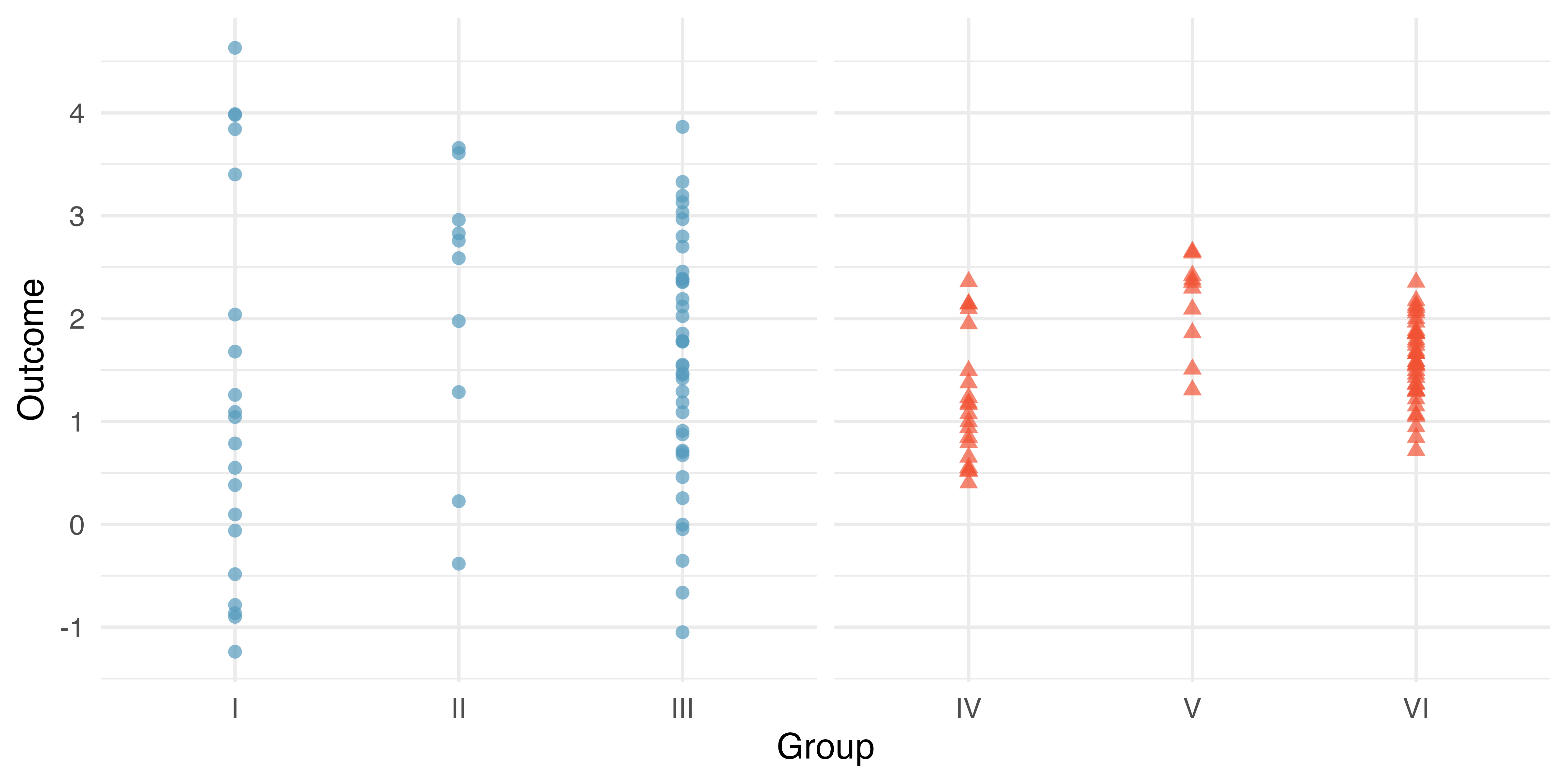
Examine Figure 22.1. Compare groups I, II, and III. Can you visually determine if the differences in the group centers is unlikely to have occurred if there were no differences in the groups? Now compare groups IV, V, and VI. Do these differences appear to be unlikely to have occurred if there were no differences in the groups?
Any real difference in the means of groups I, II, and III is difficult to discern, because the data within each group are very volatile relative to any differences in the average outcome. On the other hand, it appears there are differences in the centers of groups IV, V, and VI. For instance, group V appears to have a higher mean than that of the other two groups. Investigating groups IV, V, and VI, we see the differences in the groups’ centers are noticeable because those differences are large relative to the variability in the individual observations within each group.
22.1 Case study: Batting
We would like to discern whether there are real differences between the batting performance of baseball players according to their position: outfielder (OF), infielder (IF), and catcher (C). We will use a dataset called mlb_players_18, which includes batting records of 429 Major League Baseball (MLB) players from the 2018 season who had at least 100 at bats. Six of the 429 cases represented in mlb_players_18 are shown in Table 22.1, and descriptions for each variable are provided in Table 22.2. The measure we will use for the player batting performance (the outcome variable) is on-base percentage (OBP). The on-base percentage roughly represents the fraction of the time a player successfully gets on base or hits a home run.
The mlb_players_18 data can be found in the openintro R package.
mlb_players_18 data frame.
| name | team | position | AB | H | HR | RBI | AVG | OBP |
|---|---|---|---|---|---|---|---|---|
| Abreu, J | CWS | IF | 499 | 132 | 22 | 78 | 0.265 | 0.325 |
| Acuna Jr., R | ATL | OF | 433 | 127 | 26 | 64 | 0.293 | 0.366 |
| Adames, W | TB | IF | 288 | 80 | 10 | 34 | 0.278 | 0.348 |
| Adams, M | STL | IF | 306 | 73 | 21 | 57 | 0.239 | 0.309 |
| Adduci, J | DET | IF | 176 | 47 | 3 | 21 | 0.267 | 0.290 |
| Adrianza, E | MIN | IF | 335 | 84 | 6 | 39 | 0.251 | 0.301 |
mlb_players_18 dataset.
| Variable | Description |
|---|---|
| name | Player name |
| team | The abbreviated name of the player's team |
| position | The player's primary field position (OF, IF, C) |
| AB | Number of opportunities at bat |
| H | Number of hits |
| HR | Number of home runs |
| RBI | Number of runs batted in |
| AVG | Batting average, which is equal to H/AB |
| OBP | On-base percentage, which is roughly equal to the fraction of times a player gets on base or hits a home run |
The null hypothesis under consideration is the following: \(\mu_{OF} = \mu_{IF} = \mu_{C} % = \mu_{DH}.\) Write the null and corresponding alternative hypotheses in plain language.1
The player positions have been divided into three groups: outfield (OF), infield (IF), and catcher (C). What would be an appropriate point estimate of the on-base percentage by outfielders, \(\mu_{OF}\)?
A good estimate of the on-base percentage by outfielders would be the sample average of OBP for just those players whose position is outfield: \(\bar{x}_{OF} = 0.320.\)
22.2 Randomization test for comparing many means
Table 22.3 provides summary statistics for each group. A side-by-side box plots for the on-base percentage is shown in Figure 22.2. Notice that the variability appears to be approximately constant across groups; nearly constant variance across groups is an important assumption that must be satisfied before we consider the ANOVA approach.
| Position | n | Mean | SD |
|---|---|---|---|
| OF | 160 | 0.320 | 0.043 |
| IF | 205 | 0.318 | 0.038 |
| C | 64 | 0.302 | 0.038 |
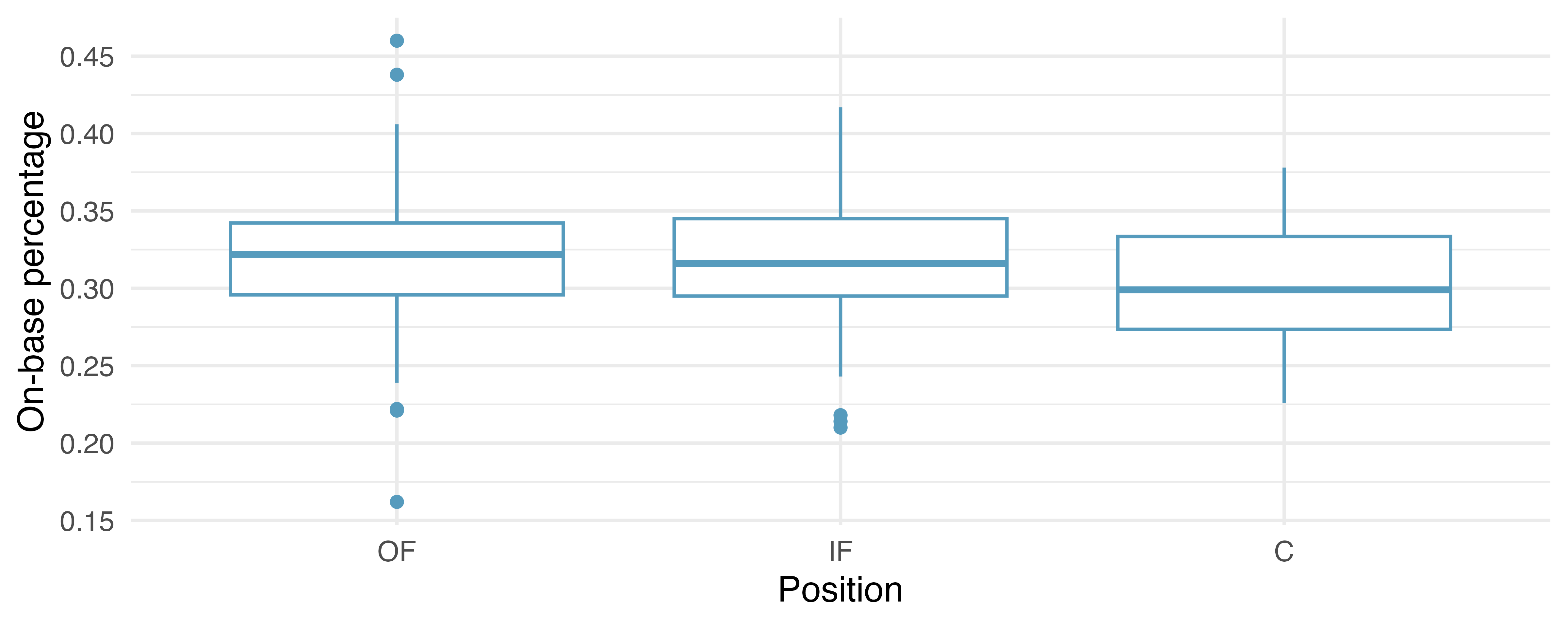
The largest difference between the sample means is between the catcher and the outfielder positions. Consider again the original hypotheses:
- \(H_0:\) \(\mu_{OF} = \mu_{IF} = \mu_{C}\)
- \(H_A:\) The average on-base percentage \((\mu_j)\) varies across some (or all) groups.
Why might it be inappropriate to run the test by simply estimating whether the difference of \(\mu_{C}\) and \(\mu_{OF}\) is “statistically discernible” at a 0.05 discernibility level?
The primary issue here is that we are inspecting the data before picking the groups that will be compared. It is inappropriate to examine all data by eye (informal testing) and only afterwards decide which parts to formally test. This is called data snooping or data fishing. Naturally, we would pick the groups with the large differences for the formal test, and this would lead to an inflation in the Type I error rate. To understand inflated Type I error rates better, let’s consider a slightly different problem.
Suppose we are to measure the aptitude for students in 20 classes in a large elementary school at the beginning of the year. In this school, all students are randomly assigned to classrooms, so any differences we observe between the classes at the start of the year are completely due to chance. However, with so many groups, we will probably observe a few groups that look rather different from each other. If we select only the classes that look different and then perform a formal test, we will probably make the wrong conclusion that the assignment wasn’t random. While we might only formally test differences for a few pairs of classes, we informally evaluated the other classes by eye before choosing the most extreme cases for a comparison.
22.2.1 Observed data
In the next section we will learn how to use the \(F\) statistic to test whether observed differences in sample means could have happened just by chance even if there was no difference in the respective population means.
The method of analysis of variance in this context focuses on answering one question: is the variability in the sample means so large that it seems unlikely to be from chance alone? This question is different from earlier testing procedures since we will simultaneously consider many groups, and evaluate whether their sample means differ more than we would expect from natural variation. We call this variability the mean square between groups (MSG) \((MSG)\), and it has an associated degrees of freedom, \(df_{G} = k - 1\) when there are \(k\) groups. The \(MSG\) can be thought of as a scaled variance formula for means. If the null hypothesis is true, any variation in the sample means is due to chance and shouldn’t be too large. Details of \(MSG\) calculations are provided in the footnote.2 However, we typically use software for these computations.
The mean square between the groups is, on its own, quite useless in a hypothesis test. We need a benchmark value for how much variability should be expected among the sample means if the null hypothesis is true. To this end, we compute a pooled variance estimate, often abbreviated as the mean square error \((MSE)\), which has an associated degrees of freedom value \(df_E = n - k.\) It is helpful to think of \(MSE\) as a measure of the variability within the groups. Details of the computations of the \(MSE\) and a link to an extra online section for ANOVA calculations are provided in the footnote.3
When the null hypothesis is true, any differences among the sample means are only due to chance, and the \(MSG\) and \(MSE\) should be about equal. As a test statistic for ANOVA, we examine the fraction of \(MSG\) and \(MSE:\)
\[F = \frac{MSG}{MSE}\]
The \(MSG\) represents a measure of the between-group variability, and \(MSE\) measures the variability within each of the groups.
The test statistic for three or more means is an F.
The F statistic is a ratio of how the groups differ (MSG) as compared to how the observations within a group vary (MSE).
\[F = \frac{MSG}{MSE}\]
When the null hypothesis is true and the conditions are met, F has an F-distribution with \(df_1 = k-1\) and \(df_2 = n-k.\)
Conditions:
- independent observations, both within and across groups
- large samples and no extreme outliers
22.2.2 Variability of the statistic
We recall the exams from Section 20.1 which demonstrated a two-sample randomization test for a comparison of means. Suppose now that the teacher had had such an extremely large class that three different exams were given: A, B, and C. Table 22.4 and Figure 22.3 provide a summary of the data including exam C. Again, we would like to investigate whether the difficulty of the exams is the same across the three exams, so the test is
- \(H_0: \mu_A = \mu_B = \mu_C.\) The inherent average difficulty is the same across the three exams.
- \(H_A:\) not \(H_0.\) At least one of the exams is inherently more (or less) difficult than the others.
| Exam | n | Mean | SD | Min | Max |
|---|---|---|---|---|---|
| A | 58 | 75.1 | 13.9 | 44 | 100 |
| B | 55 | 72.0 | 13.8 | 38 | 100 |
| C | 51 | 78.9 | 13.1 | 45 | 100 |
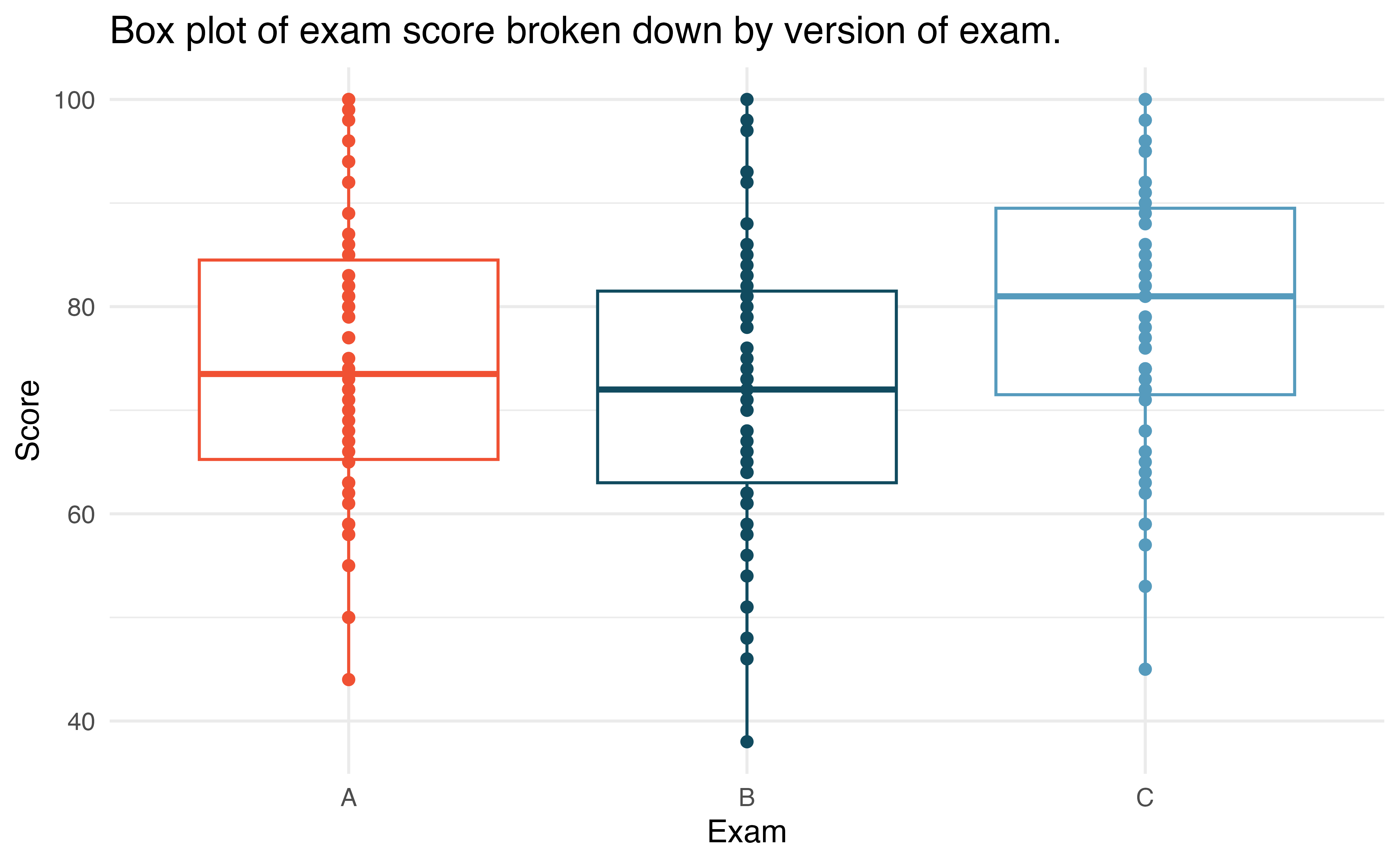
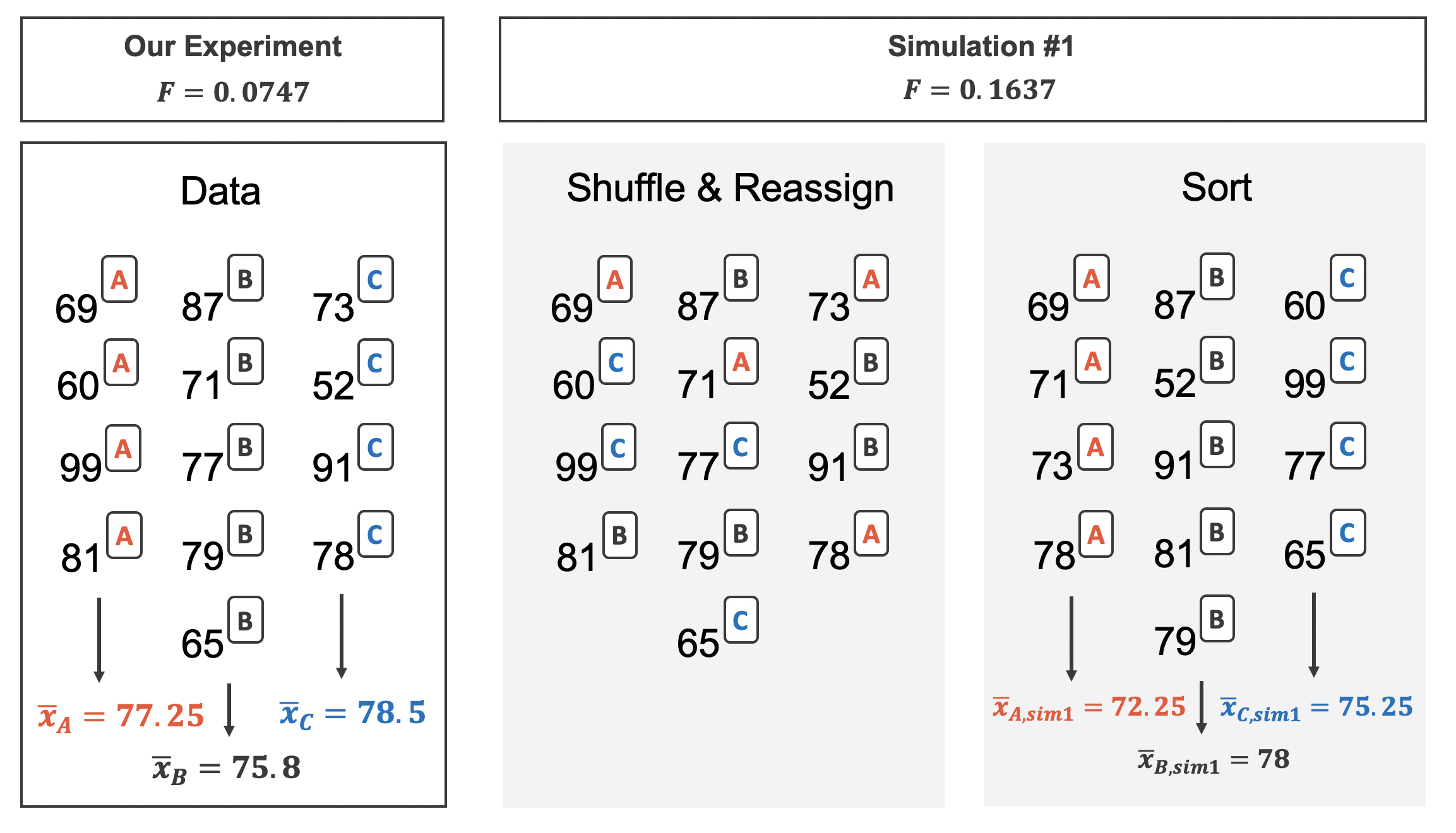
Figure 22.4 shows the process of randomizing the three different exams to the observed exam scores. If the null hypothesis is true, then the score on each exam should represent the true student ability on that material. It shouldn’t matter whether they were given exam A or exam B or exam C. By reallocating which student got which exam, we are able to understand how the difference in average exam scores changes due only to natural variability. There is only one iteration of the randomization process in Figure 22.4, leading to three different randomized sample means (computed assuming the null hypothesis is true).
In the two-sample case, the null hypothesis was investigated using the difference in the sample means. However, as noted above, with three groups (three different exams), the comparison of the three sample means gets slightly more complicated. We have already derived the F-statistic which is exactly the way to compare the averages across three or more groups! Recall, the F statistic is a ratio of how the groups differ (MSG) as compared to how the observations within a group vary (MSE).
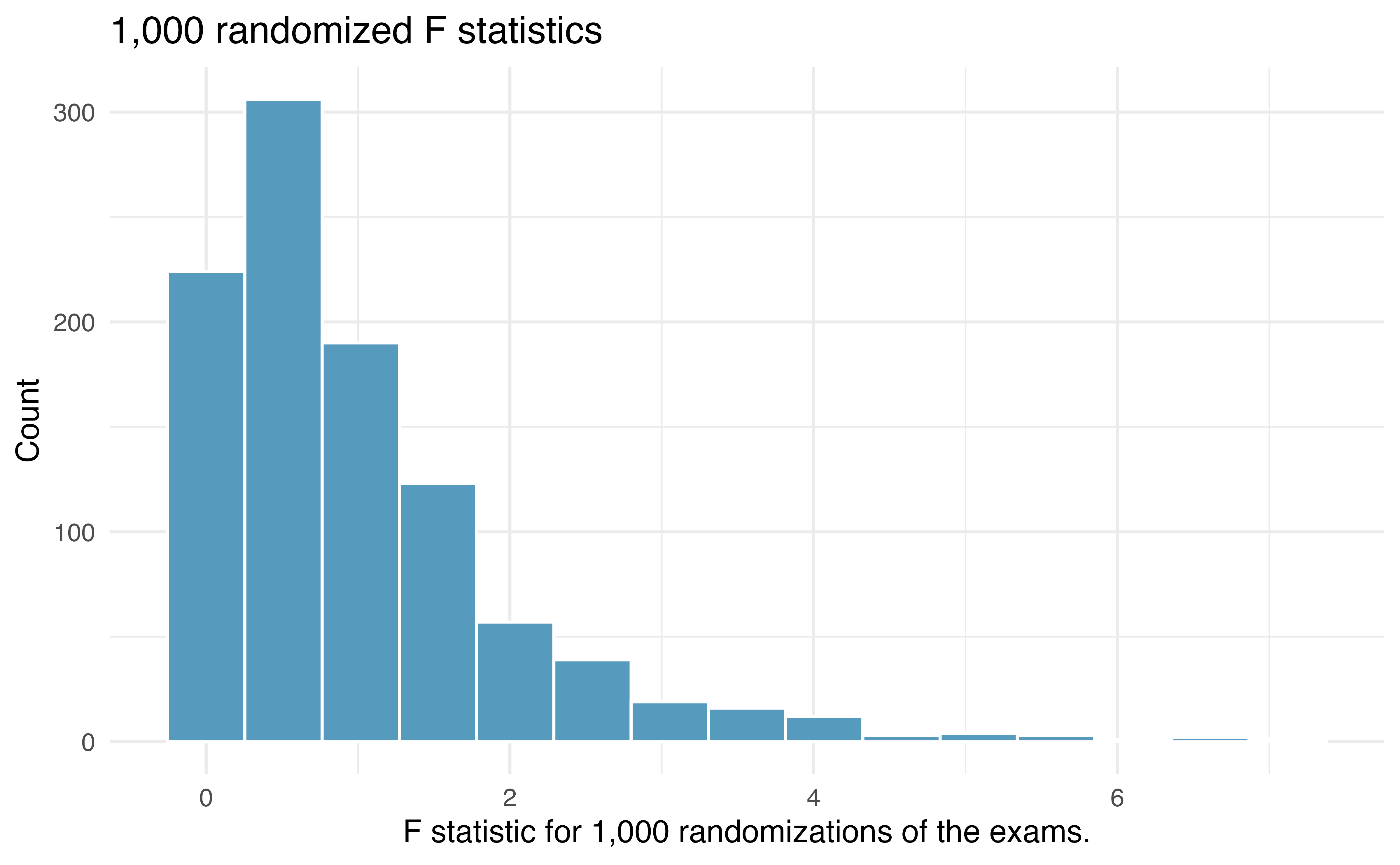
Building on Figure 22.4, Figure 22.5 shows the values of the simulated \(F\) statistics over 1,000 random simulations. We see that, just by chance, the F statistic can be as large as 7.
22.2.3 Observed statistic vs. null statistics
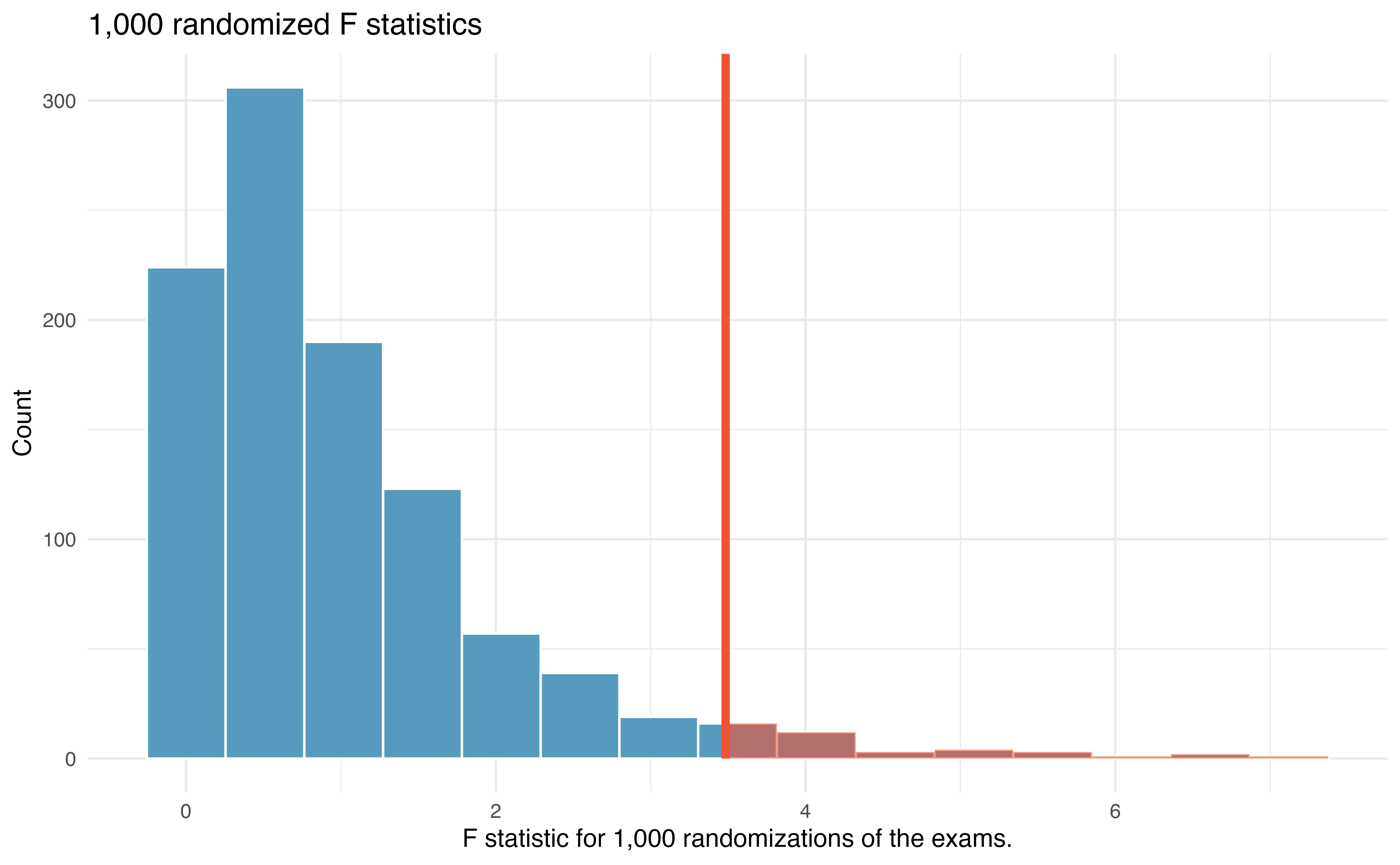
Using statistical software, we can calculate that 3.6% of the randomized F test statistics were at or above the observed test statistic of \(F= 3.48.\) That is, the p-value of the test is 0.036. Assuming that we had set the level of discernibility to be \(\alpha = 0.05,\) the p-value is smaller than the level of discernibility which would lead us to reject the null hypothesis. We claim that the difficulty level (i.e., the true average score, \(\mu)\) is different for at least one of the exams.
While it is temping to say that exam C is harder than the other two (given the inability to differentiate between exam A and exam B in Section 20.1), we must be very careful about conclusions made using different techniques on the same data.
When the null hypothesis is true, random variability that exists in nature sometimes produces data with p-values less than 0.05. How often does that happen? 5% of the time. That is to say, if you use 20 different models applied to the same data where there is no signal (i.e., the null hypothesis is true), you are reasonably likely to get a p-value less than 0.05 in one of the tests you run. The details surrounding the ideas of this problem, called a multiple comparisons test or multiple comparisons problem, are outside the scope of this textbook, but should be something that you keep in the back of your head. To best mitigate any extra Type I errors, we suggest that you set up your hypotheses and testing protocol before running any analyses. Once the conclusions have been reached, you should report your findings instead of running a different type of test on the same data.
22.3 Mathematical model for test for comparing many means
As seen with many of the tests and statistics from previous sections, the randomization test on the F statistic has corresponding mathematical theory to describe the distribution that can be used without using a computational approach.
We return to the baseball example from Table 22.3 to demonstrate the mathematical model applied to the ANOVA setting.
22.3.1 Variability of the statistic
The larger the observed variability in the sample means \((MSG)\) relative to the within-group observations \((MSE)\), the larger \(F\)-statistic will be and the stronger the evidence against the null hypothesis. Because larger \(F\)-statistics represent stronger evidence against the null hypothesis, we use the upper tail of the distribution to compute a p-value.
The F statistic and the F-test.
Analysis of variance (ANOVA) is used to test whether the mean outcome differs across two or more groups. ANOVA uses a test statistic, the \(F\)-statistic, which represents a standardized ratio of variability in the sample means relative to the variability within the groups. If \(H_0\) is true and the model conditions are satisfied, an \(F\)-statistic follows an \(F\) distribution with parameters \(df_{1} = k - 1\) and \(df_{2} = n - k.\) The upper tail of the \(F\) distribution is used to represent the p-value.
For the baseball data, \(MSG = 0.00803\) and \(MSE=0.00158\). Identify the degrees of freedom associated with MSG and MSE and verify the \(F\)-statistic is approximately 5.077.4
22.3.2 Observed statistic vs. null statistics
We can use the \(F\)-statistic to evaluate the hypotheses in what is called an F-test. A p-value can be computed from the \(F\) statistic using an \(F\) distribution, which has two associated parameters: \(df_{1}\) and \(df_{2}.\) For the \(F\)-statistic in ANOVA, \(df_{1} = df_{G}\) and \(df_{2} = df_{E}.\) An \(F\) distribution with 2 and 426 degrees of freedom, corresponding to the \(F\) statistic for the baseball hypothesis test, is shown in Figure 22.7.
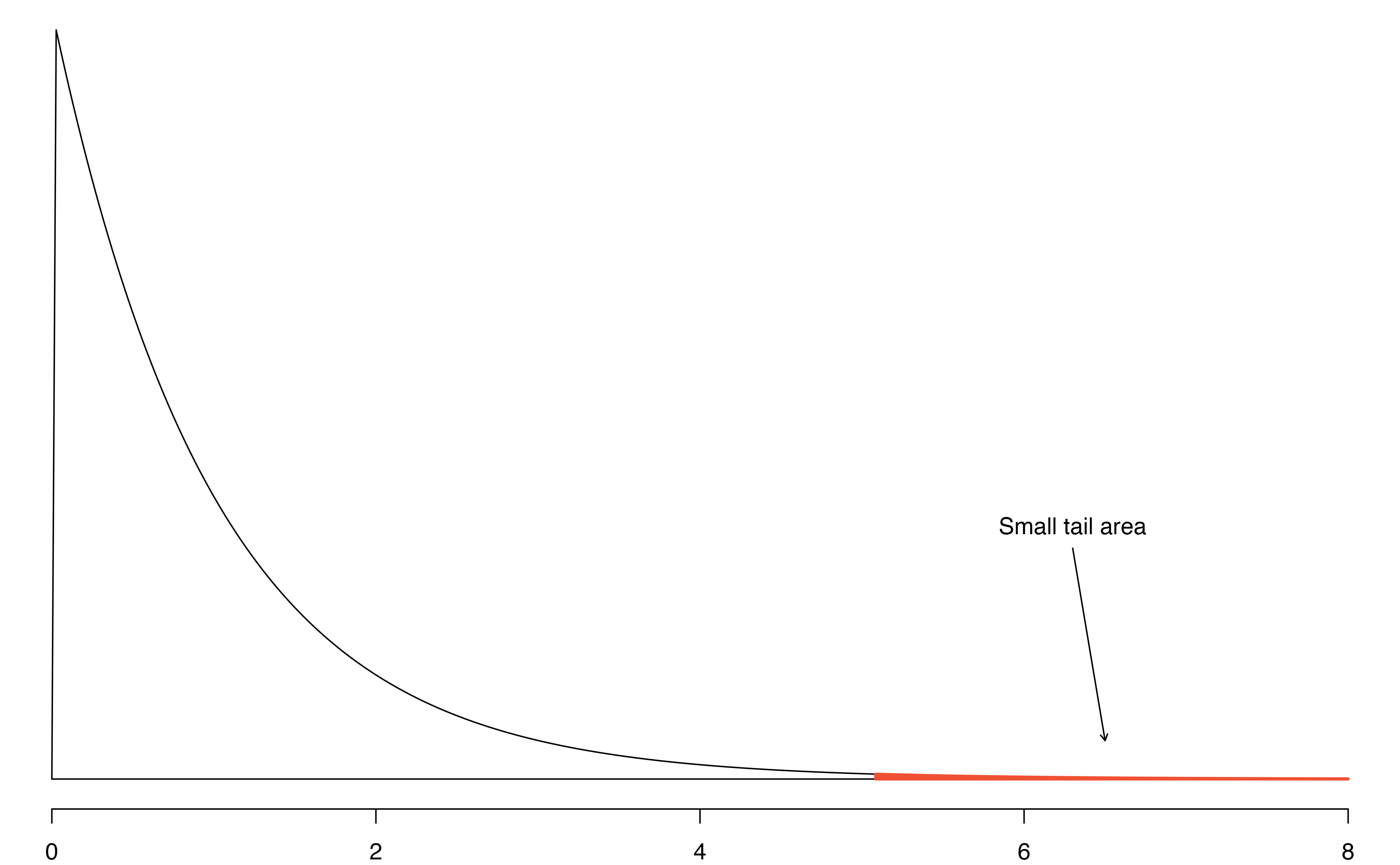
The p-value corresponding to the shaded area in Figure 22.7 is equal to about 0.0066. Does this provide strong evidence against the null hypothesis?
The p-value is smaller than 0.05, indicating the evidence is strong enough to reject the null hypothesis at a discernibility level of 0.05. That is, the data provide strong evidence that the average on-base percentage varies by player’s primary field position.
Note that the small p-value indicates that there is a notable difference between the mean batting averages of the different positions. However, the ANOVA test does not provide a mechanism for knowing which group is driving the differences. If we move forward with all possible two mean comparisons, we run the risk of a high Type I error rate. As we saw at the end of Section 22.2, the follow-up questions surrounding individual group comparisons is called a problem of multiple comparisons and is outside the scope of this text. We encourage you to learn more about multiple comparisons, however, so that additional comparisons, after you have rejected the null hypothesis in an ANOVA test, do not lead to undue false positive conclusions.
22.3.3 Reading an ANOVA table from software
The calculations required to perform an ANOVA by hand are tedious and prone to human error. For these reasons, it is common to use statistical software to calculate the \(F\)-statistic and p-value.
An ANOVA analysis can be summarized in a table very similar to that of a regression summary, which we saw in Chapter 7 and Chapter 8. Table 22.5 shows an ANOVA summary to test whether the mean of on-base percentage varies by player positions in the MLB. Many of these values should look familiar; in particular, the \(F\)-statistic and p-value can be retrieved from the last two columns.
| term | df | sumsq | meansq | statistic | p.value |
|---|---|---|---|---|---|
| position | 2 | 0.0161 | 0.0080 | 5.08 | 0.0066 |
| Residuals | 426 | 0.6740 | 0.0016 |
22.3.4 Conditions for an ANOVA analysis
There are three conditions we must check for an ANOVA analysis: all observations must be independent, the data in each group must be nearly normal (or each group must have reasonably large sample sizes), and the variance within each group must be approximately equal.
Independence. If the data are a simple random sample, this condition can be assumed to be satisfied. For processes and experiments, carefully consider whether the data may be independent (e.g., no pairing). For example, in the MLB data, the data were not sampled. However, there are not obvious reasons why independence would not hold for most or all observations.
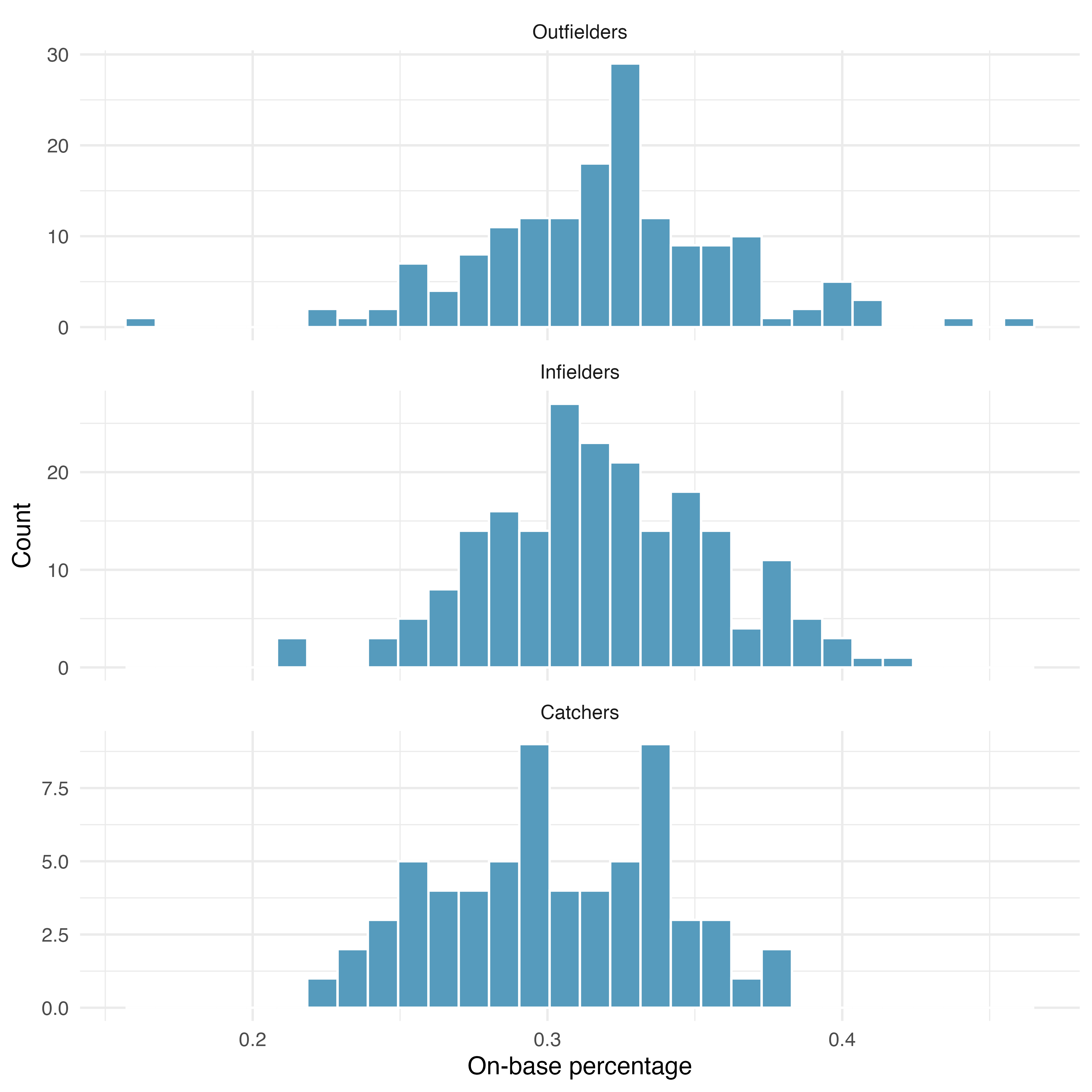
Approximately normal. As with one- and two-sample testing for means, the normality assumption is especially important when the sample size is quite small when it is ironically difficult to check for non-normality. A histogram of the observations from each group is shown in Figure 22.8. Since each of the groups we are considering have relatively large sample sizes, what we are looking for are major outliers. None are apparent, so this conditions is reasonably met.
Constant variance. The last assumption is that the variance in the groups is about equal from one group to the next. This assumption can be checked by examining side-by-side box plots of the outcomes across the groups, as in Figure 22.2. In this case, the variability is similar in the four groups but not identical. We see in Table 22.3 that the standard deviation does not vary much from one group to the next.
Diagnostics for an ANOVA analysis.
Independence is always important to an ANOVA analysis. The normality condition is important when the sample sizes for each group are relatively small (if the group sizes are large, the observations do not need to be normal but should also not contain any large outliers). The constant variance condition is especially important when the sample sizes differ between groups.
22.4 Chapter review
22.4.1 Summary
In this chapter we have provided both the randomization test and the mathematical model appropriate for addressing questions of equality of means across two or more groups. Note that there were important technical conditions required for confirming that the F distribution appropriately modeled the ANOVA test statistic. Also, you may have noticed that there was no discussion of creating confidence intervals. That is because the ANOVA statistic does not have a direct analogue parameter to estimate. If there is interest in comparisons of mean differences (across each set of two groups), then the methods from Chapter 20 comparing two independent means should be applied.
22.4.2 Terms
The terms introduced in this chapter are presented in Table 22.6. If you’re not sure what some of these terms mean, we recommend you go back in the text and review their definitions. You should be able to easily spot them as bolded text.
| analysis of variance | degrees of freedom | multiple comparisons |
| ANOVA | F-test | sum of squared error (SSE) |
| data fishing | mean square between groups (MSG) | sum of squares between groups (SSG) |
| data snooping | mean square error (MSE) | sum of squares total (SST) |
22.5 Exercises
Answers to odd-numbered exercises can be found in Appendix A.22.
- Fill in the blank. When doing an ANOVA, you observe large differences in means between groups. Within the ANOVA framework, this would most likely be interpreted as evidence strongly favoring the _____________ hypothesis.
- Which test? We would like to test if students who are in the social sciences, natural sciences, arts and humanities, and other fields spend the same amount of time, on average, studying for a course. What type of test should we use? Explain your reasoning.
-
Cuckoo bird egg lengths, randomize once. Cuckoo birds lay their eggs in other birds’ nests, making them known as brood parasites. One question relates to whether the size of the cuckoo egg differs depending on the species of the host bird.5 (Latter 1902) Consider the following plots, one represents the original data, the second represents data where the host species has been randomly assigned to the egg length.
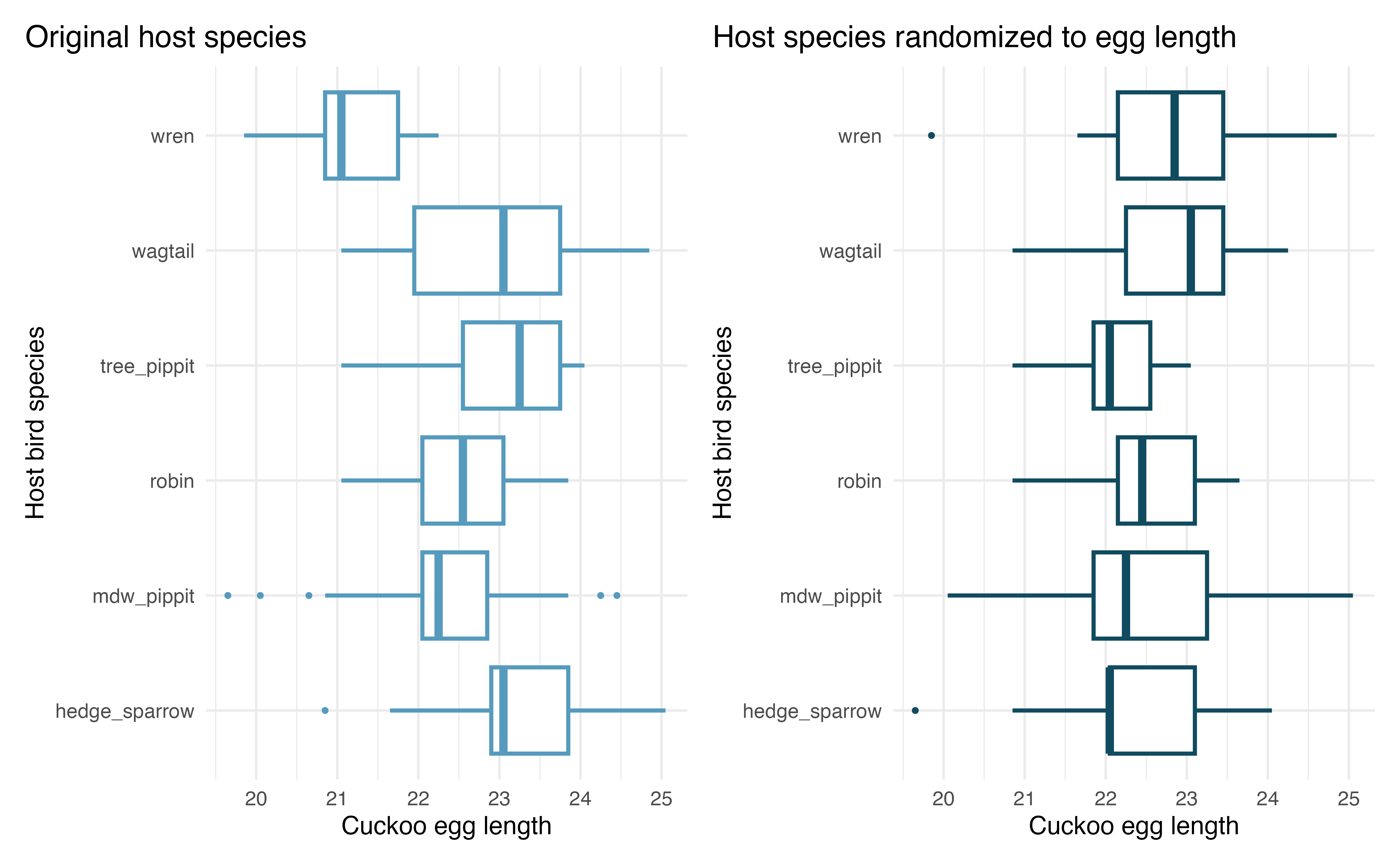
Consider the average length of the eggs for each species. Is the average length for the original data: more variable, less variable, or about the same as the randomized species? Describe what you see in the plots.
Consider the standard deviation of the lengths of the eggs within each species. Is the within species standard deviation of the length for the original data: bigger, smaller, or about the same as the randomized species?
Recall that the F statistic’s numerator measures how much the groups vary (MSG) with the denominator measuring how much the within species values vary (MSE), which of the plots above would have a larger F statistic, the original data or the randomized data? Explain.
-
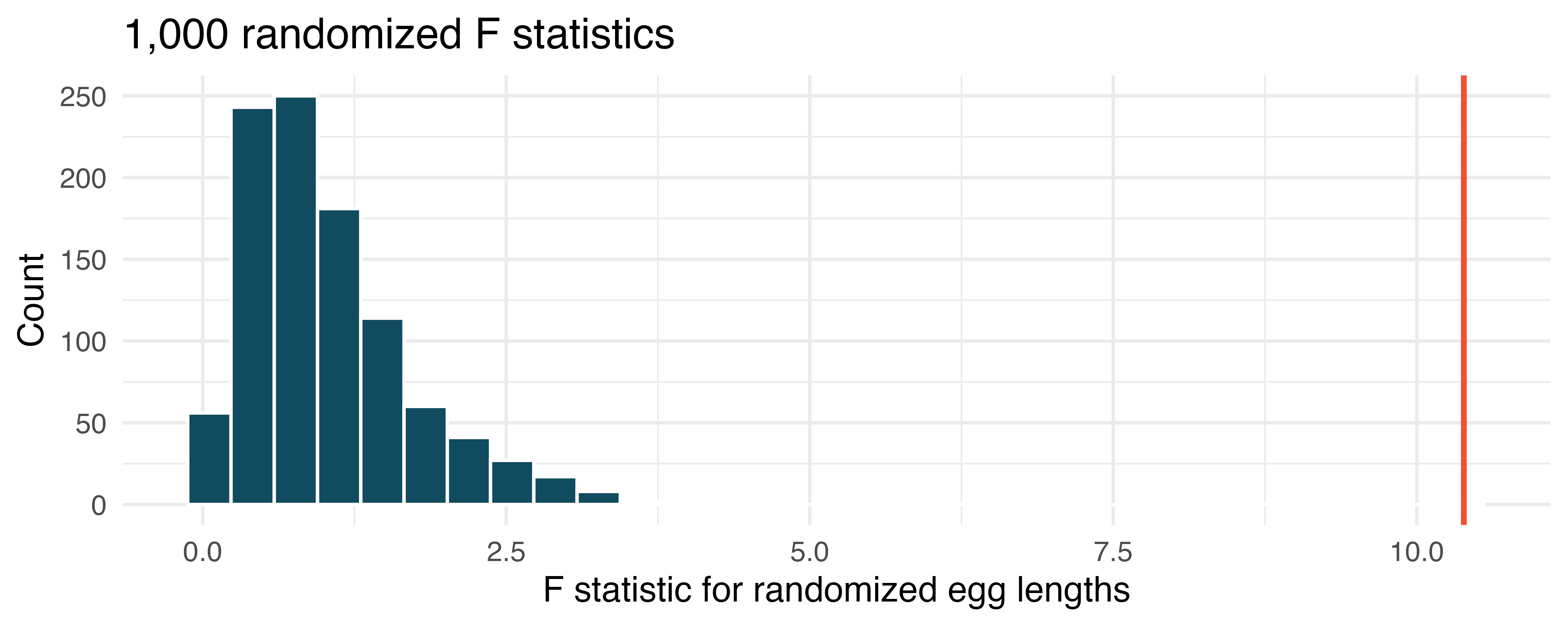
Cuckoo bird egg lengths, randomization test. Cuckoo birds lay their eggs in other birds’ nests, making them known as brood parasites. One question relates to whether the size of the cuckoo egg differs depending on the species of the host bird.6 (Latter 1902) Using the randomization distribution of the F statistic (host species randomized to egg length), conduct a hypothesis test to evaluate if there is a difference, in the population, between the average egg lengths for different host bird species. Make sure to state your hypotheses clearly and interpret your results in context of the data.
-
Chicken diet and weight, many groups. An experiment was conducted to measure and compare the effectiveness of various feed supplements on the growth rate of chickens. Newly hatched chicks were randomly allocated into six groups, and each group was given a different feed supplement. Sample statistics and a visualization of the observed data are shown below. (McNeil 1977)
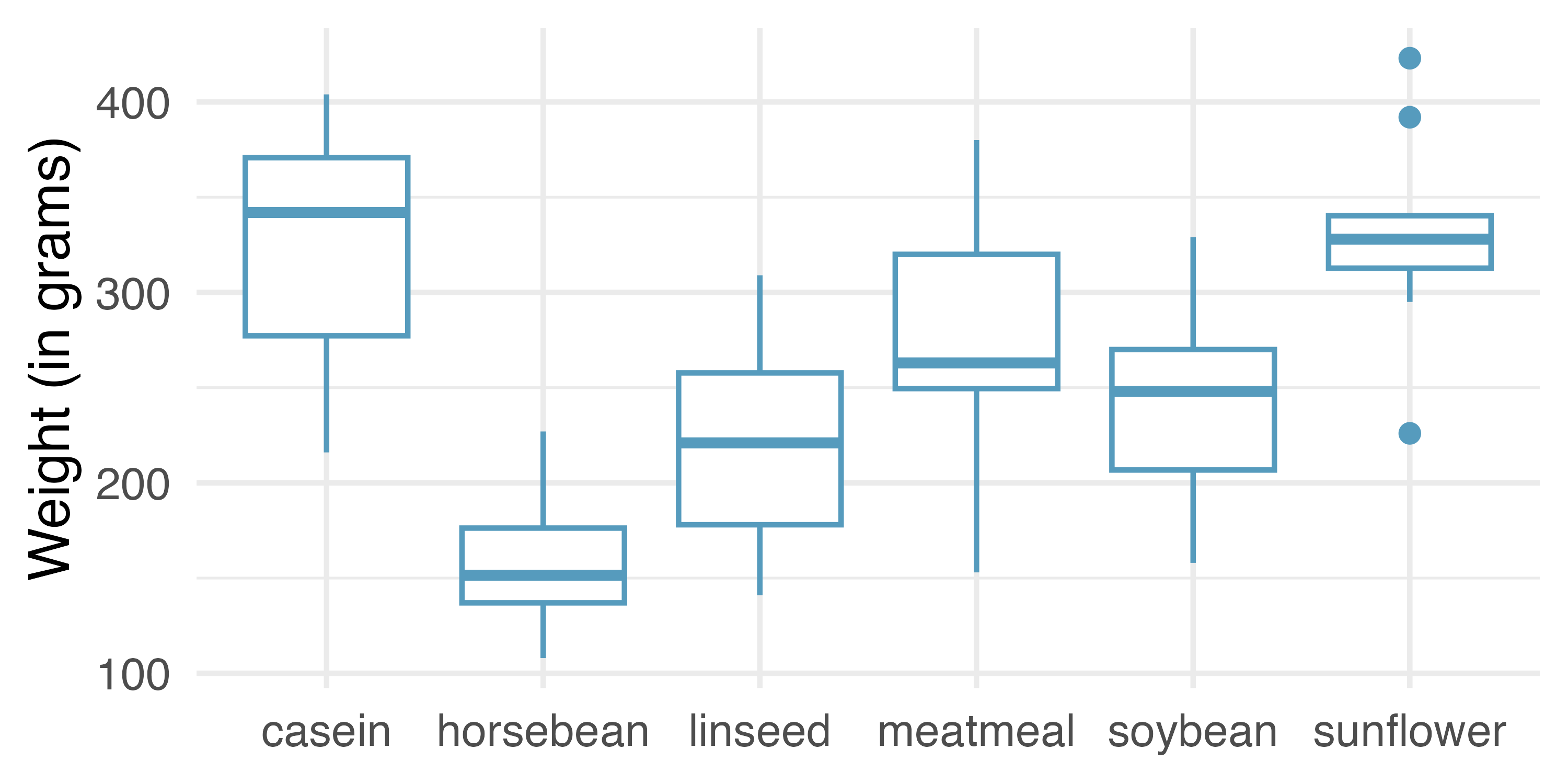
Feed type Mean SD n casein 323.58 64.43 12 horsebean 160.20 38.63 10 linseed 218.75 52.24 12 meatmeal 276.91 64.90 11 soybean 246.43 54.13 14 sunflower 328.92 48.84 12 Using the ANOVA output below, conduct a hypothesis test to determine if these data provide convincing evidence that the average weight of chicks varies across some (or all) groups. Make sure to check relevant conditions.
term df sumsq meansq statistic p.value feed 5 231,129 46,226 15.4 <0.0001 Residuals 65 195,556 3,009
-
Teaching descriptive statistics. A study compared five different methods for teaching descriptive statistics. The five methods were traditional lecture and discussion, programmed textbook instruction, programmed text with lectures, computer instruction, and computer instruction with lectures. 45 students were randomly assigned, 9 to each method. After completing the course, students took a 1-hour exam.
What are the hypotheses for evaluating if the average test scores are different for the different teaching methods?
What are the degrees of freedom associated with the \(F\)-test for evaluating these hypotheses?
Suppose the p-value for this test is 0.0168. What is the conclusion?
-
Coffee, depression, and physical activity. Caffeine is the world’s most widely used stimulant, with approximately 80% consumed in the form of coffee. Participants in a study investigating the relationship between coffee consumption and exercise were asked to report the number of hours they spent per week on moderate (e.g., brisk walking) and vigorous (e.g., strenuous sports and jogging) exercise. Based on these data the researchers estimated the total hours of metabolic equivalent tasks (MET) per week, a value always greater than 0. The table below gives summary statistics of MET for women in this study based on the amount of coffee consumed. (Lucas et al. 2011)
1 cup / week or fewer 2-6 cups / week 1 cups / day 2-3 cups / day 4 cups / day or more Mean 18.7 19.6 19.3 18.9 17.5 SD 21.1 25.5 22.5 22.0 22.0 n 12,215.0 6,617.0 17,234.0 12,290.0 2,383.0 Write the hypotheses for evaluating if the average physical activity level varies among the different levels of coffee consumption.
Check conditions and describe any assumptions you must make to proceed with the test.
Below is the output associated with this test. What is the conclusion of the test?
df sumsq meansq statistic p.value cofee 4 10,508 2,627 5.2 0 Residuals 50,734 25,564,819 504 Total 50,738 25,575,327
-
Student performance across discussion sections. A professor who teaches a large introductory statistics class (197 students) with eight discussion sections would like to test if student performance differs by discussion section, where each discussion section has a different teaching assistant. The summary table below shows the average final exam score for each discussion section as well as the standard deviation of scores and the number of students in each section.
Sec 1 Sec 2 Sec 3 Sec 4 Sec 5 Sec 6 Sec 7 Sec 8 Mean 92.94 91.11 91.80 92.45 89.30 88.30 90.12 93.35 SD 4.21 5.58 3.43 5.92 9.32 7.27 6.93 4.57 n 33.00 19.00 10.00 29.00 33.00 10.00 32.00 31.00 The ANOVA output below can be used to test for differences between the average scores from the different discussion sections.
df sumsq meansq statistic p.value section 7 525 75.0 1.87 0.077 Residuals 189 7,584 40.1 Total 196 8,109 Conduct a hypothesis test to determine if these data provide convincing evidence that the average score varies across some (or all) groups. Check conditions and describe any assumptions you must make to proceed with the test.
-
GPA and major. Undergraduate students in an introductory statistics course at Duke University conducted a survey about GPA and major. The density plots show the distributions of GPA among three groups of majors. ANOVA output is also provided.
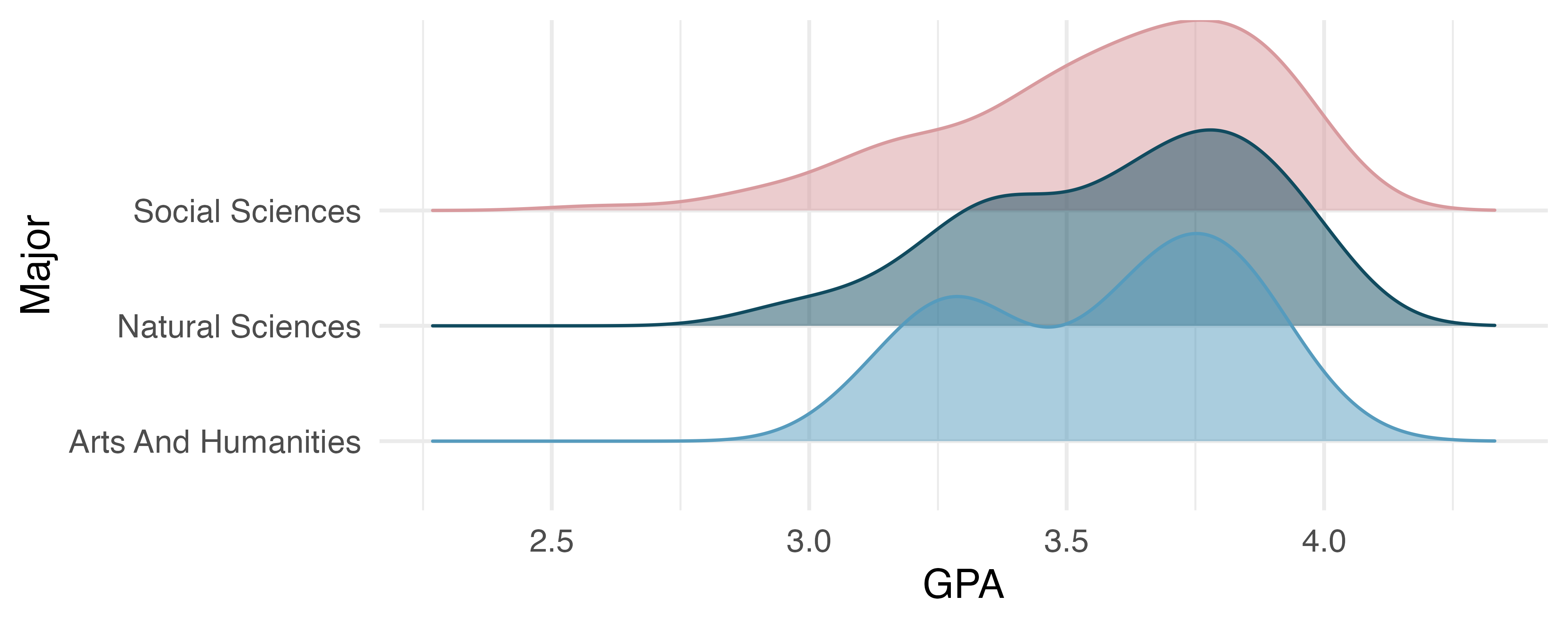
term df sumsq meansq statistic p.value major 2 0.03 0.02 0.21 0.81 Residuals 195 15.77 0.08 Write the hypotheses for testing for a difference between average GPA across majors.
What is the conclusion of the hypothesis test?
How many students answered the questions on the survey, i.e., what is the sample size?
-
Work hours and education. The General Social Survey collects data on demographics, education, and work, among many other characteristics of US residents. (NORC 2010) Using ANOVA, we can consider educational attainment levels for all 1,172 respondents at once. Below are the distributions of hours worked by educational attainment and relevant summary statistics that will be helpful in carrying out this analysis.
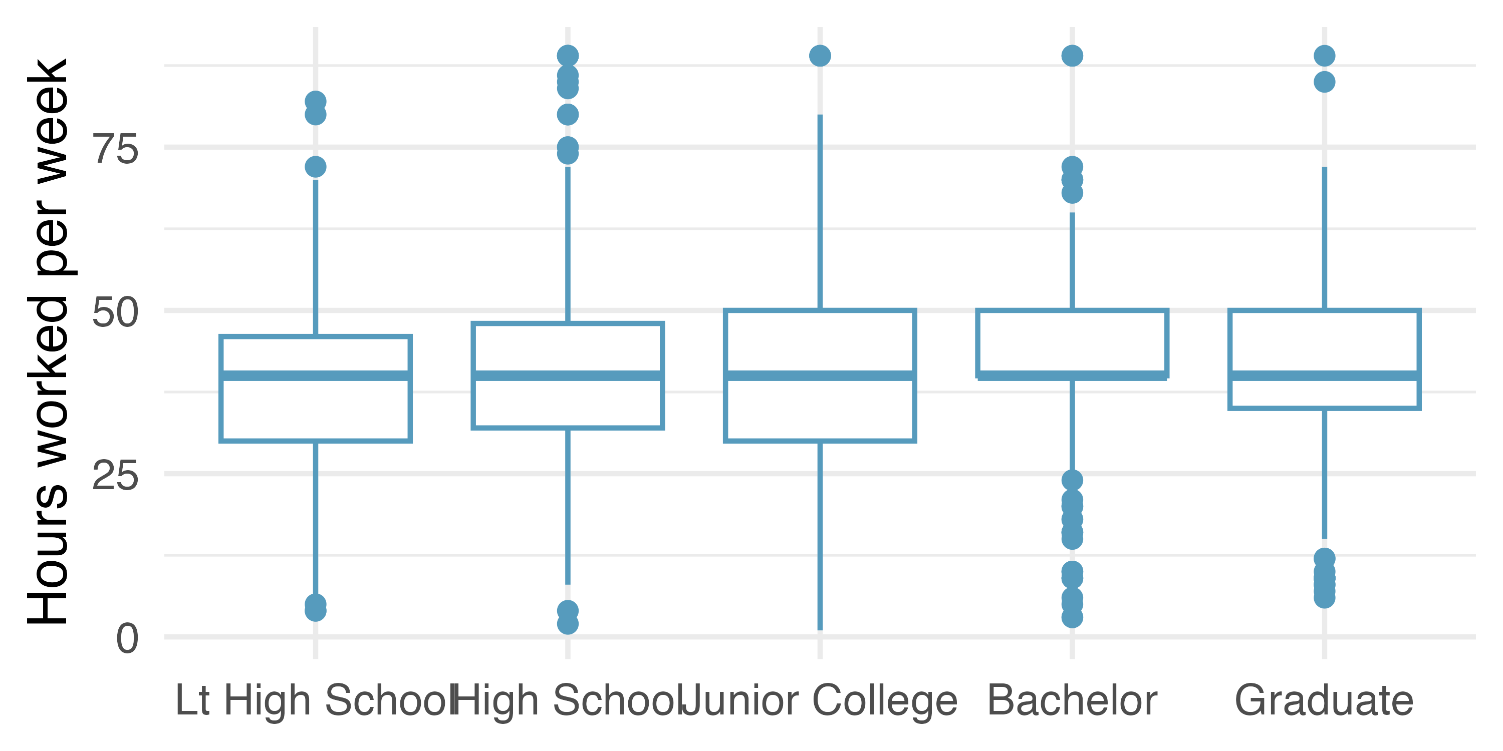
Educational attainment Mean SD n Lt High School 38.7 15.8 121 High School 39.6 15.0 546 Junior College 41.4 18.1 97 Bachelor 42.5 13.6 253 Graduate 40.8 15.5 155 Write hypotheses for evaluating whether the average number of hours worked varies across the five groups.
Check conditions and describe any assumptions you must make to proceed with the test.
Below is the output associated with this test. What is the conclusion of the test?
term df sumsq meansq statistic p.value degree 4 2,006 502 2.19 0.07 Residuals 1,167 267,382 229
-
True / False: ANOVA, I. Determine if the following statements are true or false in ANOVA, and explain your reasoning for statements you identify as false.
As the number of groups increases, the modified discernibility level for pairwise tests increases as well.
As the total sample size increases, the degrees of freedom for the residuals increases as well.
The constant variance condition can be somewhat relaxed when the sample sizes are relatively consistent across groups.
The independence assumption can be relaxed when the total sample size is large.
-
True / False: ANOVA, II. Determine if the following statements are true or false, and explain your reasoning for statements you identify as false.
If the null hypothesis that the means of four groups are all the same is rejected using ANOVA at a 5% discernibility level, then…
we can then conclude that all the means are different from one another.
the standardized variability between groups is higher than the standardized variability within groups.
the pairwise analysis will identify at least one pair of means that are discernibly different.
the appropriate \(\alpha\) to be used in pairwise comparisons is 0.05 / 4 = 0.0125 since there are four groups.
-
Matching observed data with randomized F statistics. Consider the following two datasets. The response variable is the
scoreand the explanatory variable is whether the individual is in one of four groups.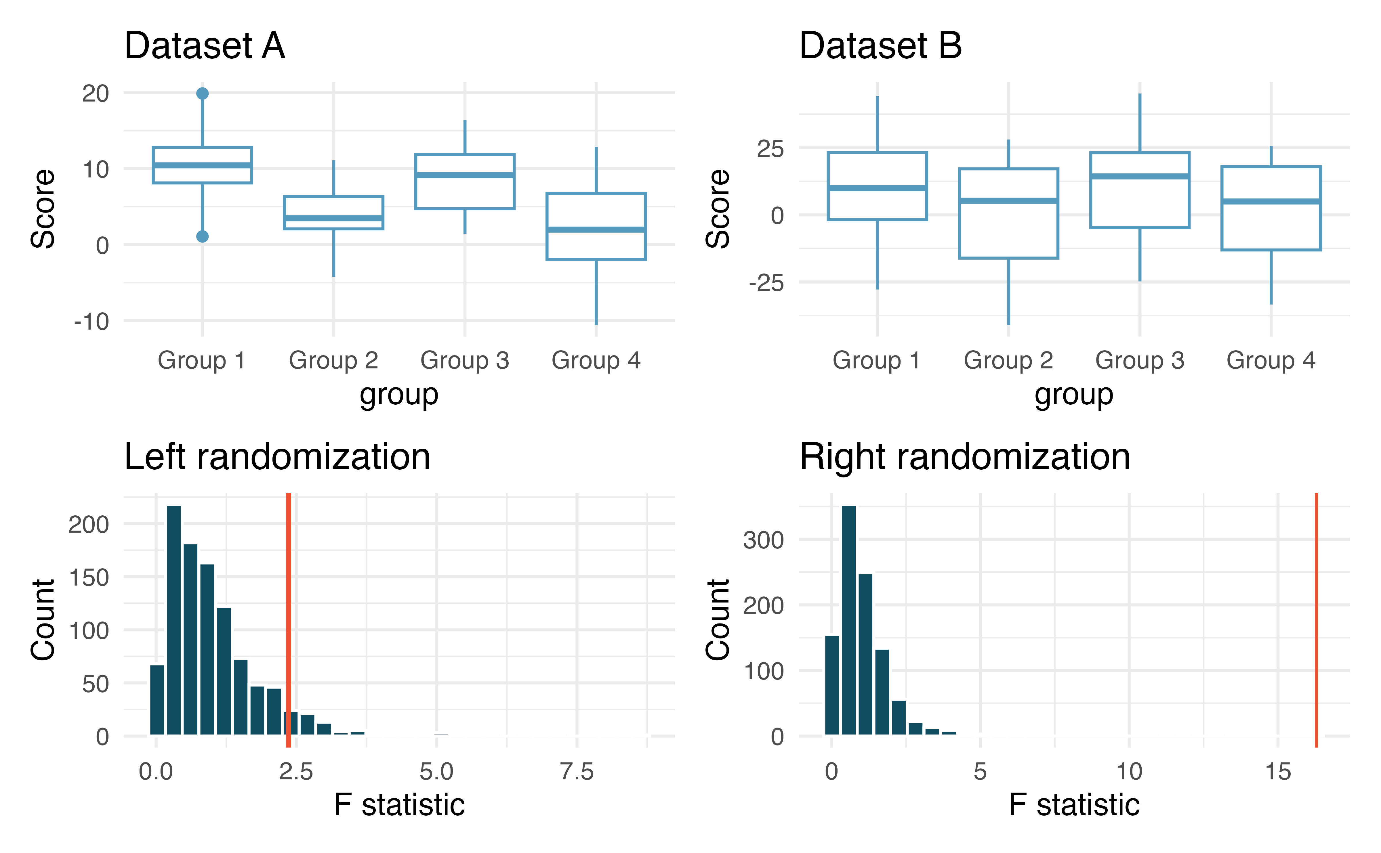
The randomizations (randomly assigning group to the score, calculating a randomization F statistic) were done 1000 times for each of Dataset A and B. The red line on each plot indicates the observed F statistic for the original (unrandomized) data.
Does the randomization distribution on the left correspond to Dataset A or B? Explain.
Does the randomization distribution on the right correspond to Dataset A or B? Explain.
-
Child care hours. The China Health and Nutrition Survey aims to examine the effects of the health, nutrition, and family planning policies and programs implemented by national and local governments. (UNC Carolina Population Center 2006) It, for example, collects information on number of hours Chinese parents spend taking care of their children under age 6. The side-by-side box plots below show the distribution of this variable by educational attainment of the parent. Also provided below is the ANOVA output for comparing average hours across educational attainment categories.
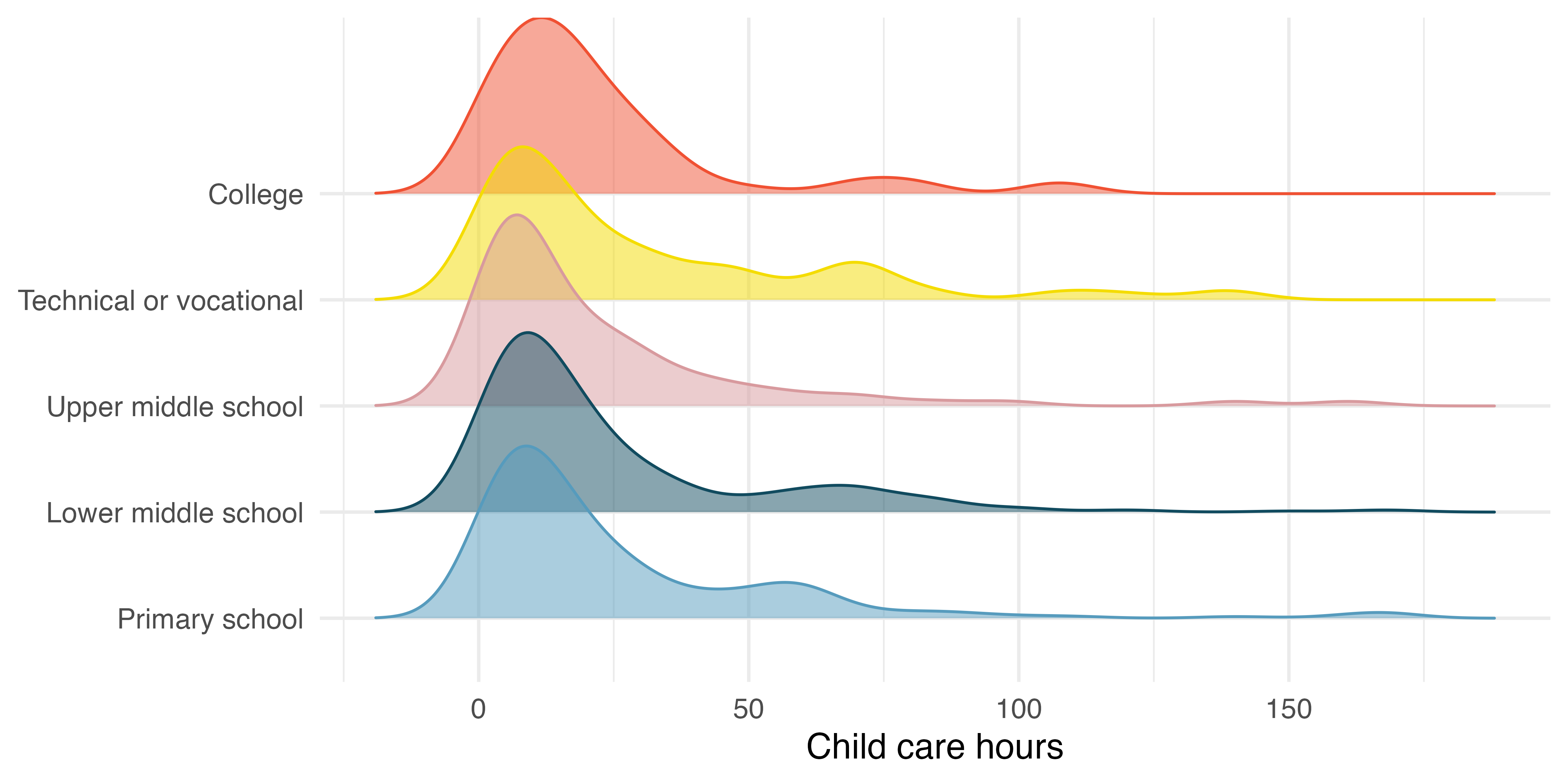
term df sumsq meansq statistic p.value edu 4 4,142 1,036 1.26 0.28 Residuals 794 653,048 822 Write the hypotheses for testing for a difference between the average number of hours spent on child care across educational attainment levels.
What is the conclusion of the hypothesis test?
\(H_0:\) The average on-base percentage is equal across the four positions. \(H_A:\) The average on-base percentage varies across some (or all) groups.↩︎
Let \(\bar{x}\) represent the mean of outcomes across all groups. Then the mean square between groups is computed as \(MSG = \frac{1}{df_{G}}SSG = \frac{1}{k-1}\sum_{j=1}^{k} n_{j} \left(\bar{x}_{j} - \bar{x}\right)^2\) where \(SSG\) is called the sum of squares between groups \((SSG)\) and \(n_{j}\) is the sample size of group \(j.\)↩︎
See additional details on ANOVA calculations for interested readers. Let \(\bar{x}\) represent the mean of outcomes across all groups. Then the sum of squares total \((SST)\) is computed as \[SST = \sum_{i=1}^{n} \left(x_{i} - \bar{x}\right)^2\] where the sum is over all observations in the dataset. Then we compute the sum of squared errors \((SSE)\) in one of two equivalent ways: \(SSE = SST - SSG = (n_1-1)s_1^2 + (n_2-1)s_2^2 + \cdots + (n_k-1)s_k^2\) where \(s_j^2\) is the sample variance (square of the standard deviation) of the residuals in group \(j.\) Then the \(MSE\) is the standardized form of \(SSE: MSE = \frac{1}{df_{E}}SSE.\)↩︎
There are \(k = 3\) groups, so \(df_{G} = k - 1 = 2.\) There are \(n = n_1 + n_2 + n_3 = 429\) total observations, so \(df_{E} = n - k = 426.\) Then the \(F\)-statistic is computed as the ratio of \(MSG\) and \(MSE:\) \(F = \frac{MSG}{MSE} = \frac{0.00803}{0.00158} = 5.082 \approx 5.077.\) \((F = 5.077\) was computed by using values for \(MSG\) and \(MSE\) that were not rounded.)↩︎
The
Cuckoodata used in this exercise can be found in the Stat2Data R package.↩︎The data
Cuckooused in this exercise can be found in the Stat2Data R package.↩︎