23 Applications: Infer
23.1 Recap: Computational methods
The computational methods we have presented are used in two settings. First, in many real life applications (as in those covered here), the mathematical model and computational model give identical conclusions. When there are no differences in conclusions, the advantage of the computational method is that it gives the analyst a good sense for the logic of the statistical inference process. Second, when there is a difference in the conclusions (seen primarily in methods beyond the scope of this text), it is often the case that the computational method relies on fewer technical conditions and is therefore more appropriate to use.
23.1.1 Randomization
An important feature of randomization tests is that the data are permuted in such a way that the null hypothesis is true. The randomization distribution provides a distribution of the statistic of interest under the null hypothesis, which is exactly the information needed to calculate a p-value — where the p-value is the probability of obtaining the observed data or more extreme when the null hypothesis is true. Although there are ways to adjust the randomization for settings other than the null hypothesis being true, they are not covered in this book and they are not used widely. In approaching research questions with a randomization test, be sure to ask yourself what the null hypothesis represents and how it is that permuting the data is creating different possible null data representations.
Hypothesis tests. When using a randomization test, we proceed as follows:
Write appropriate hypotheses.
Compute the observed statistic of interest.
Permute the data repeatedly, each time, recalculating the statistic of interest.
Compute the proportion of times the permuted statistics are as extreme as or more extreme than the observed statistic, this is the p-value.
Make a conclusion based on the p-value, and write the conclusion in context and in plain language so anyone can understand the result.
23.1.2 Bootstrapping
Bootstrapping, in contrast to randomization tests, represents a proxy sampling of the original population. With bootstrapping, the analyst is not forcing the null hypothesis to be true (or false, for that matter), but instead, they are replicating the variability seen in taking repeated samples from a population. Because there is no underlying true (or false) null hypothesis, bootstrapping is typically used for creating confidence intervals for the parameter of interest. Bootstrapping can be used to test particular values of a parameter (e.g., by evaluating whether a particular value of interest is contained in the confidence interval), but generally, bootstrapping is used for interval estimation instead of testing.
Confidence intervals. The following is how we generally computed a confidence interval using bootstrapping:
Repeatedly resample the original data, with replacement, using the same sample size as the original data.
For each resample, calculate the statistic of interest.
-
Calculate the confidence interval using one of the following methods:
Bootstrap percentile interval: Obtain the endpoints representing the middle (e.g., 95%) of the bootstrapped statistics. The endpoints will be the confidence interval.
Bootstrap standard error (SE) interval: Find the SE of the bootstrapped statistics. The confidence interval will be given by the original observed statistic plus or minus some multiple (e.g., 2) of SEs.
Put the conclusions in context and in plain language so even non-statisticians and data scientists can understand the results.
23.2 Recap: Mathematical models
The mathematical models which have been used to produce inferential analyses follow a consistent framework for different parameters of interest. As a way to contrast and compare the mathematical approach, we offer the following summaries in Table 23.1 and Table 23.2.
23.2.1 z-procedures
Generally, when the response variable is categorical (or binary), the summary statistic is a proportion and the model used to describe the proportion is the standard normal curve (also referred to as a \(z\)-curve or a \(z\)-distribution). We provide Table 23.1 partly as a mechanism for understanding \(z\)-procedures and partly to highlight the extremely common usage of the \(z\)-distribution in practice.
| One sample | Two independent samples | |
|---|---|---|
| Response variable | Binary | Binary |
| Parameter of interest | Proportion: \(p\) | Difference in proportions: \(p_1 - p_2\) |
| Statistic of interest | Proportion: \(\widehat{p}\) | Difference in proportions: \(\widehat{p}_1 - \widehat{p}_2\) |
| Standard error: HT | \(\sqrt{\frac{p_0(1-p_0)}{n}}\) | \(\sqrt{\widehat{p}_{pool}\bigg(1-\widehat{p}_{pool}\bigg)\bigg(\frac{1}{n_1} + \frac{1}{n_2}}\bigg)\) |
| Standard error: CI | \(\sqrt{\frac{\widehat{p}(1-\widehat{p})}{n}}\) | \(\sqrt{\frac{\widehat{p}_{1}(1-\widehat{p}_{1})}{n_1} + \frac{\widehat{p}_{2}(1-\widehat{p}_{2})}{n_2}}\) |
| Conditions | 1. Independence, 2. Success-failure | 1. Independence, 2. Success-failure |
Hypothesis tests. When applying the \(z\)-distribution for a hypothesis test, we proceed as follows:
Write appropriate hypotheses.
-
Verify conditions for using the \(z\)-distribution.
- One-sample: the observations (or differences) must be independent. The success-failure condition of at least 10 success and at least 10 failures should hold.
- For a difference of proportions: each sample must separately satisfy the success-failure conditions, and the data in the groups must also be independent.
Compute the point estimate of interest and the standard error.
Compute the Z score and p-value.
Make a conclusion based on the p-value, and write a conclusion in context and in plain language so anyone can understand the result.
Confidence intervals. Similarly, the following is how we generally computed a confidence interval using a \(z\)-distribution:
- Verify conditions for using the \(z\)-distribution. (See above.)
- Compute the point estimate of interest, the standard error, and \(z^{\star}.\)
- Calculate the confidence interval using the general formula:
point estimate \(\pm\ z^{\star} SE.\) - Put the conclusions in context and in plain language so even non-statisticians and data scientists can understand the results.
23.2.2 t-procedures
With quantitative response variables, the \(t\)-distribution was applied as the appropriate mathematical model in three distinct settings. Although the three data structures are different, their similarities and differences are worth pointing out. We provide Table 23.2 partly as a mechanism for understanding \(t\)-procedures and partly to highlight the extremely common usage of the \(t\)-distribution in practice.
| One sample | Paired samples | Two independent samples | |
|---|---|---|---|
| Response variable | Numeric | Numeric | Numeric |
| Parameter of interest | Mean: \(\mu\) | Paired mean: \(\mu_{diff}\) | Difference in means: \(\mu_1 - \mu_2\) |
| Statistic of interest | Mean: \(\bar{x}\) | Paired mean: \(\bar{x}_{diff}\) | Difference in means: \(\bar{x}_1 - \bar{x}_2\) |
| Standard error | \(\frac{s}{\sqrt{n}}\) | \(\frac{s_{diff}}{\sqrt{n_{diff}}}\) | \(\sqrt{\frac{s_1^2}{n_1} + \frac{s_2^2}{n_2}}\) |
| Degrees of freedom | \(n-1\) | \(n_{diff} -1\) | \(\min(n_1 -1, n_2 - 1)\) |
| Conditions | 1. Independence, 2. Normality or large samples | 1. Independence, 2. Normality or large samples | 1. Independence, 2. Normality or large samples |
Hypothesis tests. When applying the \(t\)-distribution for a hypothesis test, we proceed as follows:
Write appropriate hypotheses.
-
Verify conditions for using the \(t\)-distribution.
- One-sample or differences from paired data: the observations (or differences) must be independent and nearly normal. For larger sample sizes, we can relax the nearly normal requirement, e.g., slight skew is okay for sample sizes of 15, moderate skew for sample sizes of 30, and strong skew for sample sizes of 60.
- For a difference of means when the data are not paired: each sample mean must separately satisfy the one-sample conditions for the \(t\)-distribution, and the data in the groups must also be independent.
Compute the point estimate of interest, the standard error, and the degrees of freedom. For \(df,\) use \(n-1\) for one sample, and for two samples use either statistical software or the smaller of \(n_1 - 1\) and \(n_2 - 1.\)
Compute the T score and p-value.
Make a conclusion based on the p-value, and write a conclusion in context and in plain language so anyone can understand the result.
Confidence intervals. Similarly, the following is how we generally computed a confidence interval using a \(t\)-distribution:
- Verify conditions for using the \(t\)-distribution. (See above.)
- Compute the point estimate of interest, the standard error, the degrees of freedom, and \(t^{\star}_{df}.\)
- Calculate the confidence interval using the general formula: \[\mbox{point estimate } \pm\ t_{df}^{\star} SE.\]
- Put the conclusions in context and in plain language so even non-statisticians and data scientists can understand the results.
23.3 Case study: Redundant adjectives
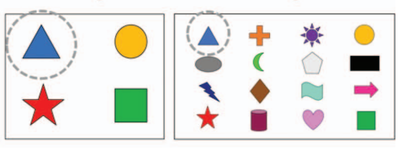
Take a look at the images in Figure 23.1. How would you describe the circled item in Figure 23.1 (a)? Would you call it “the triangle”? Or “the blue triangle”? How about in Figure 23.1 (b)? Does your answer change?


In Figure 23.1 (a) the circled item is the only triangle, but in the bottom image the circled item is one of two triangles. While in Figure 23.1 (a) “the triangle” is a sufficient description for the circled item, many of us might choose to refer to it as the “blue triangle” anyway. In Figure 23.1 (a) there are two triangles, so “the triangle” is no longer sufficient, and to describe the circled item we must qualify it with the color as well, as “the blue triangle”.
Your answers to the above questions might be different if you’re answering in a different language than English. For example, in Spanish, the adjective comes after the noun (e.g., “el triángulo azul”) therefore the incremental value of the additional adjective might be different for Figure 23.1 (a).
Researchers studying frequent use of redundant adjectives (e.g., referring to a single triangle as “the blue triangle”) and incrementality of language processing designed an experiment where they showed the following two images to 22 native English speakers (undergraduates from University College London) and 22 native Spanish speakers (undergraduates from the Universidad de las Islas Baleares). They found that in both languages, the subjects used more redundant color adjectives in denser displays where it would be more efficient. (Rubio-Fernandez et al. 2021) One of the displays from the study is shown in Figure 23.2.
In this case study we will examine data from redundant adjective study, which the authors have made available on Open Science Framework at osf.io/9hw68.
Table 23.3 shows the top six rows of the data. The full dataset has 88 rows. Remember that there are a total of 44 subjects in the study (22 English and 22 Spanish speakers). There are two rows in the dataset for each of the subjects: one representing data from when they were shown an image with 4 items on it and the other with 16 items on it. Each subject was asked 10 questions for each type of image (with a different layout of items on the image for each question). The variable of interest to us is redundant_perc, which gives the percentage of questions the subject used a redundant adjective to identify “the blue triangle”. Note that the variable is “percentage”, and we are interested in the average percentage. Therefore, we will use methods for means. If the variable had been “success or failure” (e.g., “used redundant or didn’t”), we would have used methods for proportions.
| language | subject | items | n_questions | redundant_perc |
|---|---|---|---|---|
| English | 1 | 4 | 10 | 100 |
| English | 1 | 16 | 10 | 100 |
| English | 2 | 4 | 10 | 0 |
| English | 2 | 16 | 10 | 0 |
| English | 3 | 4 | 10 | 100 |
| English | 3 | 16 | 10 | 100 |
23.3.1 Exploratory analysis
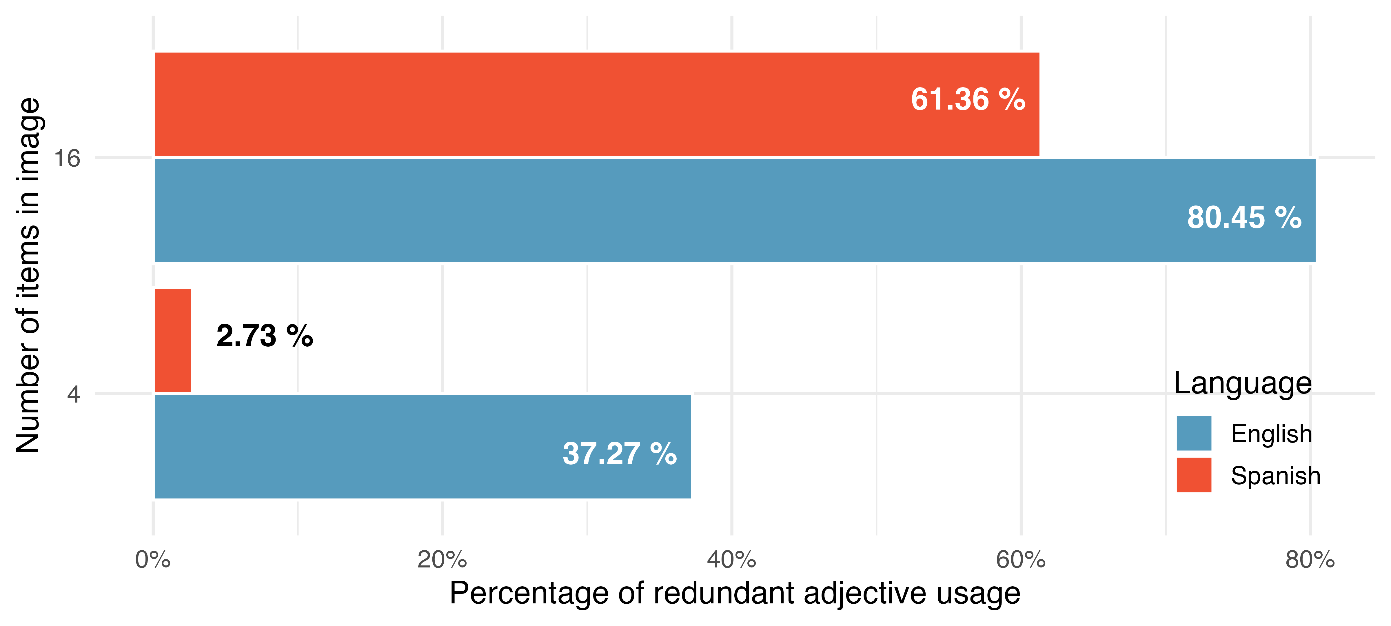
In one of the images shown to the subjects, there are 4 items, and in the other, there are 16 items. In each of the images the circled item is the only triangle, therefore referring to it as “the blue triangle” or as “el triángulo azul” is considered redundant. If the subject’s response was “the triangle”, they were recorded to have not used a redundant adjective. If the response was “the blue triangle”, they were recorded to have used a redundant adjective. Figure 23.3 shows the results of the experiment. We can see that English speakers are more likely than Spanish speakers to use redundant adjectives, and that in both languages, subjects are more likely to use a redundant adjective when there are more items in the image (i.e., in a denser display).
23.3.2 Confidence interval for a single mean
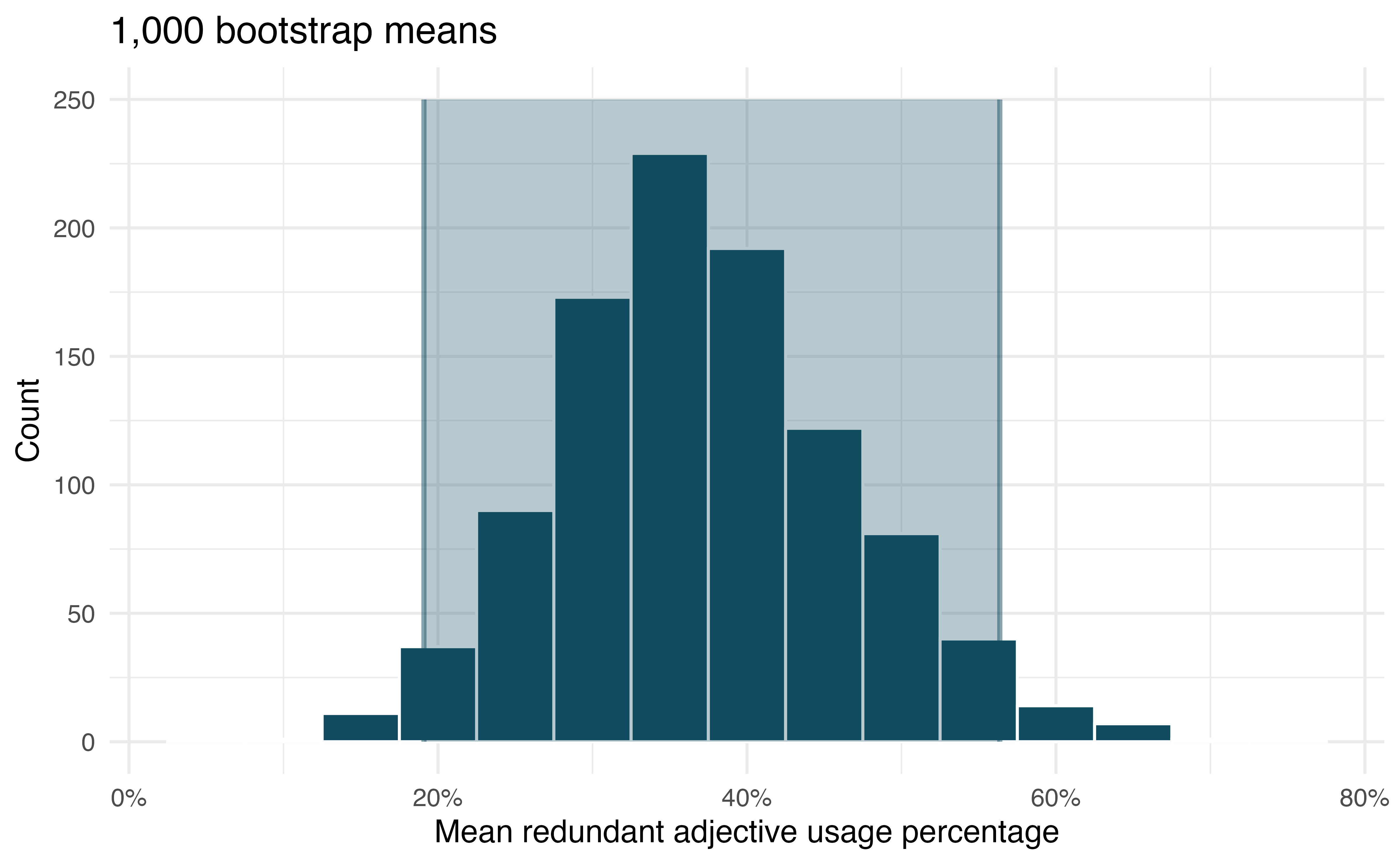
In this experiment, the average percentage of redundant adjective usage among subjects who responded in English when presented with an image with 4 items in it is 37.27. Along with the sample average as a point estimate, however, we can construct a confidence interval for the true mean redundant adjective usage of English speakers who use redundant color adjectives when describing items in an image that is not very dense.
Using a computational method, we can construct the interval via bootstrapping. Figure 23.4 shows the distribution of 1,000 bootstrapped means from this sample. The 95% confidence interval (that is calculated by taking the 2.5th and 97.5th percentile of the bootstrap distribution is 19.1% to 56.4%. Note that this interval for the true population parameter is only valid if we can assume that the sample of English speakers are representative of the population of all English speakers.
Using a similar technique, we can also construct confidence intervals for the true mean redundant adjective usage percentage for English speakers who are shown dense (16 item) displays and for Spanish speakers with both types (4 and 16 items) displays. However, these confidence intervals are not very meaningful to compare to one another as the interpretation of the “true mean redundant adjective usage percentage” is quite an abstract concept. Instead, we might be more interested in comparative questions such as “Does redundant adjective usage differ between dense and sparse displays among English speakers and among Spanish speakers?” or “Does redundant adjective usage differ between English speakers and Spanish speakers?” To answer either of these questions we need to conduct a hypothesis test.
23.3.3 Paired mean test
Let’s start with the following question: “Do the data provide convincing evidence of a difference in mean redundant adjective usage percentages between sparse (4 item) and dense (16 item) displays for English speakers?” Note that the English speaking participants were each evaluated on both the 4 item and the 16 item displays. Therefore, the variable of interest is the difference in redundant percentage. The statistic of interest will be the average of the differences, here \(\bar{x}_{diff} =\) 43.18.
Data from the first six English speaking participants are seen in Table 23.4. Although the redundancy percentages seem higher in the 16 item task, a hypothesis test will tell us whether the differences observed in the data could be due to natural variability.
| subject | redundant_perc_4 | redundant_perc_16 | diff_redundant_perc |
|---|---|---|---|
| 1 | 100 | 100 | 0 |
| 2 | 0 | 0 | 0 |
| 3 | 100 | 100 | 0 |
| 4 | 10 | 80 | 70 |
| 5 | 0 | 90 | 90 |
| 6 | 0 | 70 | 70 |
We can answer the research question using a hypothesis test with the following hypotheses:
\[H_0: \mu_{diff} = 0\] \[H_A: \mu_{diff} \ne 0\]
where \(\mu_{diff}\) is the true difference in redundancy percentages when comparing a 16 item display with a 4 item display. Recall that the computational method used to assess a hypothesis pertaining to the true average of a paired difference shuffles the observed percentage across the two groups (4 item vs 16 item) but within a single participant. The shuffling process allows for repeated calculations of potential sample differences under the condition that the null hypothesis is true.
Figure 23.5 shows the distribution of 1,000 mean differences from redundancy percentages permuted across the two conditions. Note that the distribution is centered at 0, since the structure of randomly assigning redundancy percentages to each item display will balance the data out such that the average of any differences will be zero.
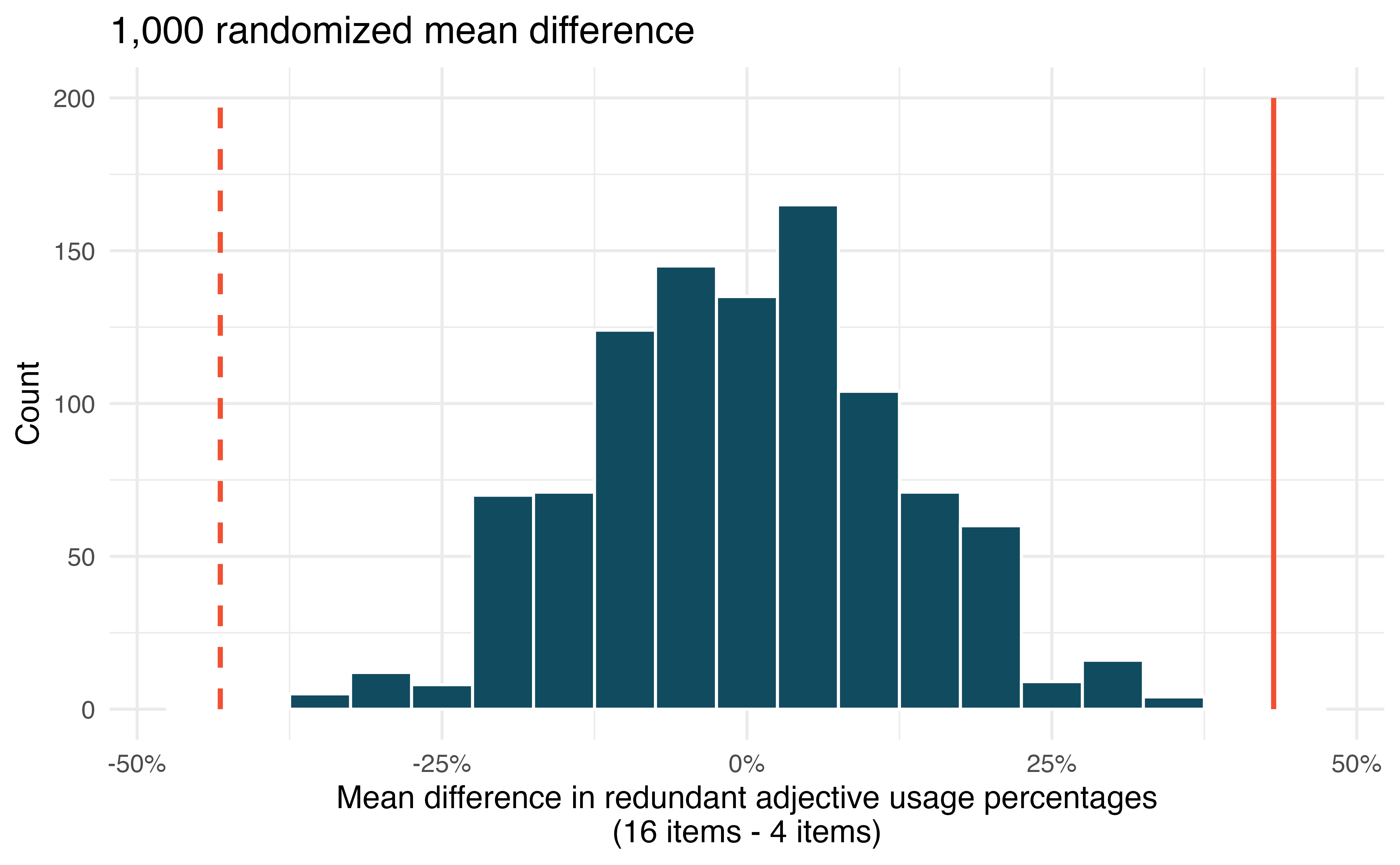
With such a small p-value, we reject the null hypothesis and conclude that the data provide convincing evidence of a difference in mean redundant adjective usage percentages across different displays for English speakers.
23.3.4 Two independent means test
Finally, let’s consider the question “How does redundant adjective usage differ between English speakers and Spanish speakers?” The English speakers are independent from the Spanish speakers, but since the same subjects were shown the two types of displays, we can’t combine data from the two display types (4 objects and 16 objects) together while maintaining independence of observations. Therefore, to answer questions about language differences, we will need to conduct two hypothesis tests, one for sparse displays and the other for dense displays. In each of the tests, the hypotheses are as follows:
\[H_0: \mu_{English} = \mu_{Spanish}\] \[H_A: \mu_{English} \ne \mu_{Spanish}\]
Here, the randomization process is slightly different than the paired setting (because the English and Spanish speakers do not have a natural pairing across the two groups). To answer the research question using a computational method, we can use a randomization test where we permute the data across all participants under the assumption that the null hypothesis is true (no difference in mean redundant adjective usage percentages across English vs Spanish speakers).
Figure 23.6 shows the null distributions for each of the two hypothesis tests. The p-value for the 4 item display comparison is very small (0.002) while the p-value for the 16 item display is much larger (0.102).
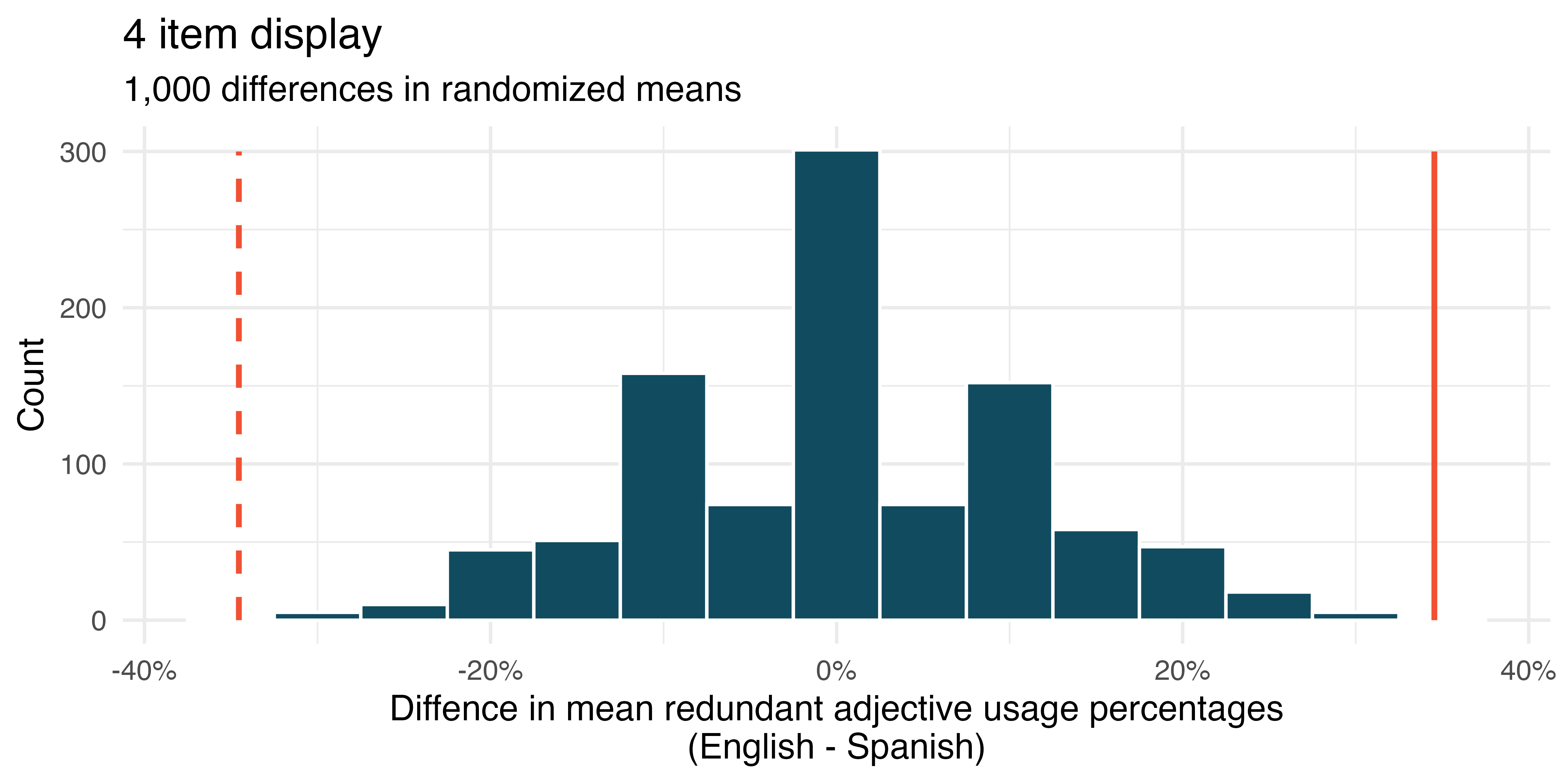
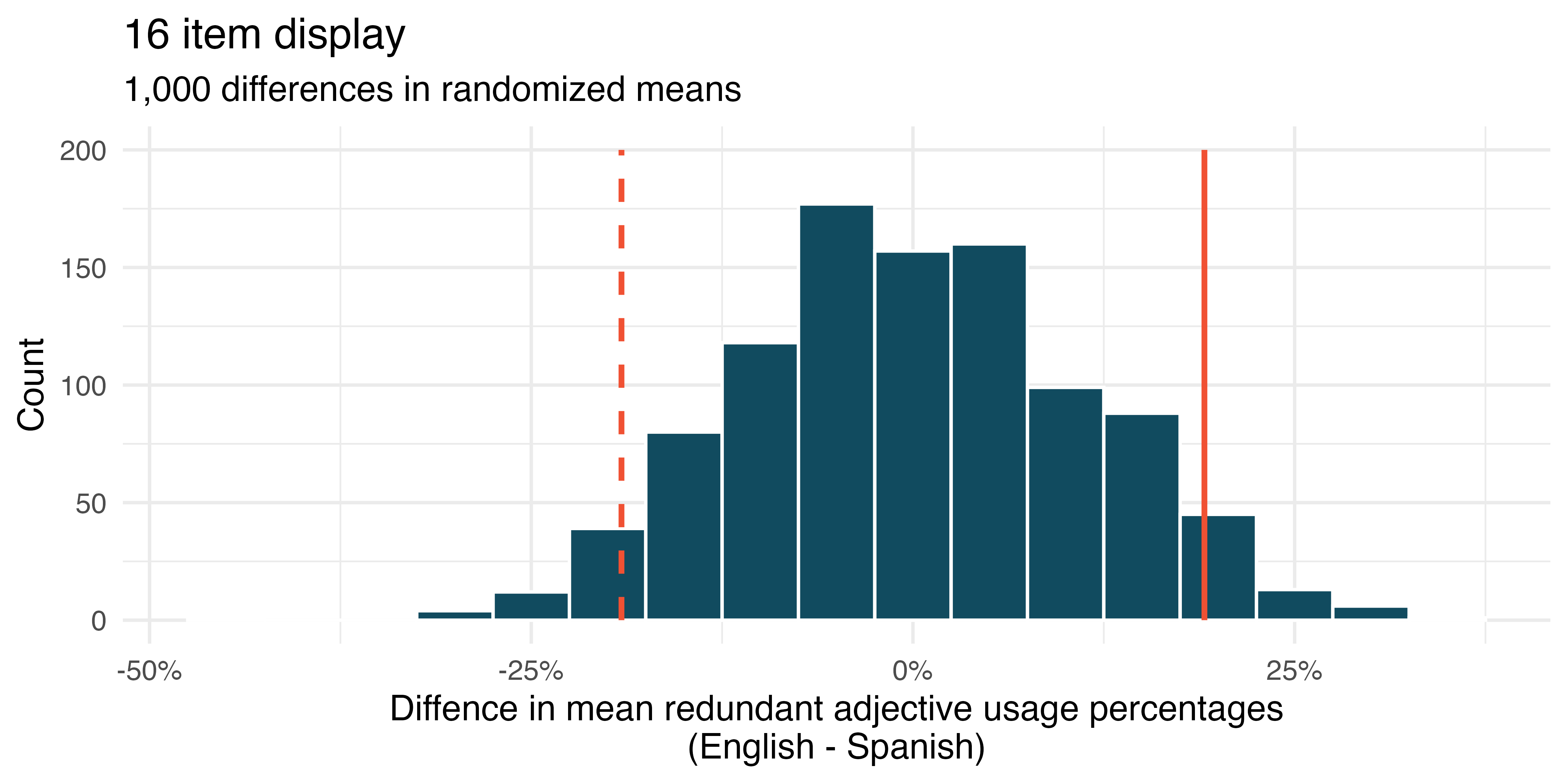
Based on the p-values (a measure of deviation from the null claim), we can conclude that the data provide convincing evidence of a difference in mean redundant adjective usage percentages between languages in 4 item displays (small p-value) but not in 16 item displays (not small p-value). The results suggests that language patterns around redundant adjective usage might be more similar for denser displays than sparser displays across English and Spanish speakers.
23.4 Interactive R tutorials
Navigate the concepts you’ve learned in this part in R using the following self-paced tutorials. All you need is your browser to get started!
You can also access the full list of tutorials supporting this book here.
23.5 R labs
Further apply the concepts you’ve learned in this part in R with computational labs that walk you through a data analysis case study.
You can also access the full list of labs supporting this book here.